Double & Triple Integrals

The goal with our vector calculus discussions is to build up to the famous Stokes’ and divergence theorems, which many consider the cornerstones of vector calculus.

These theorems have to do with integrating vector fields and the differential vector field operators over surfaces and curves.

As we know, vectors have multiple components and are usually higher dimensional objects. Therefore, we need to first understand the notion of integrals in higher dimensions before we can get to anything else.

In this lesson, however, we’ll only look at things in 1, 2 or 3 dimensions.

Lesson Contents

Double Integrals

Multivariable integrals are really just integrals in more than one dimension and they aren’t that much different from ordinary integrals of one variable. Multivariable integration is used to integrate a function of multiple variables, as you might expect.

So, with a multivariable integral, we’re really talking about integrating a scalar field (i.e. a multivariable function). We want to look at this first, since generalizing integration to vector fields (ultimately in the form of Stokes’ and divergence theorems) is based on the concept of multivariable integrals.

In 2D, a multivariable integral of a scalar field f(x,y) is a double integral over both of the variables x and y:

int_{ }^{ }int_{ }^{ }fleft(x{,}yright)dxdy

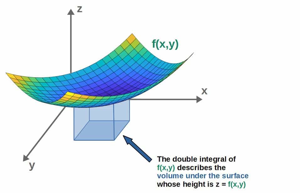
Now, remember that integrals in 1D represented the area under the function you’re integrating (the integrand).

In a similar sense, a double integral represents the volume in a region under a surface whose “height” is described by the integrand function:

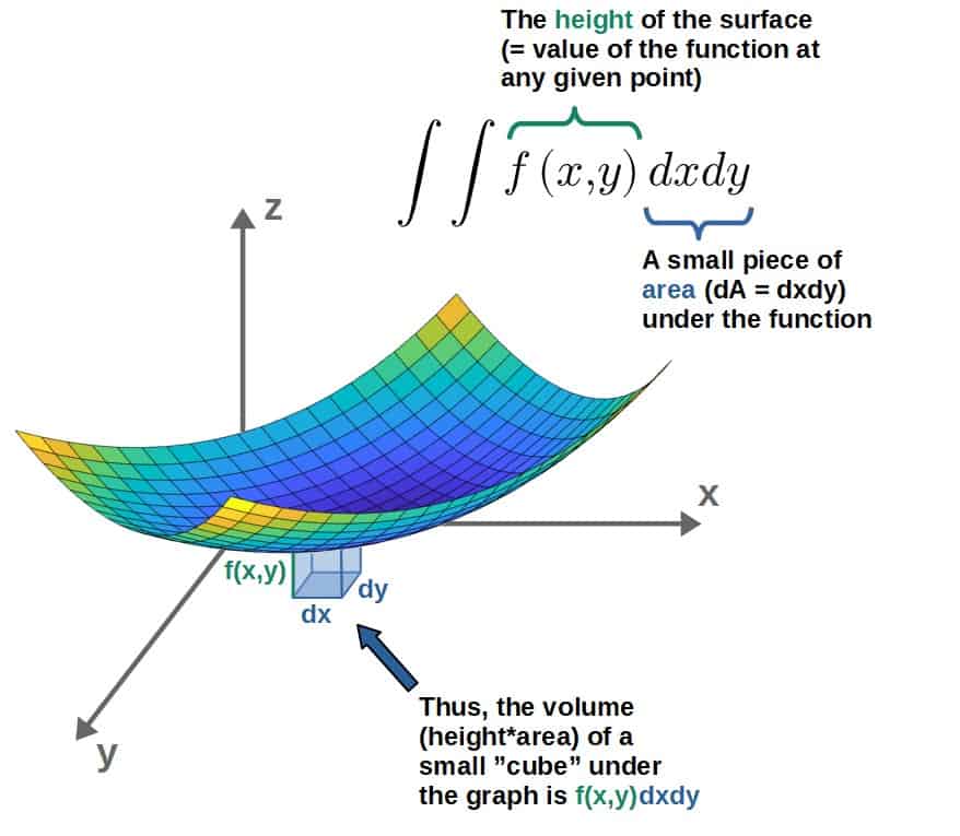
We can also understand the geometric intuition behind all of the pieces in the integral itself by breaking down the volume into little (infinitesimal) “cubes”:

An integral represents a sum, so the double integral itself would then represent summing over all of these little cubes to get the total volume under a certain region of the graph. This dxdy=dA is called an **area element**, which is basically a tiny piece of area with side lengths dx and dy.

Example: How To Do a Multivariable Integral

For example, we could have the function f(x,y)=x²-y, the integration limits of x going from 0 to 1 and the limits of y going from -1 to 1, so the double integral of this would be:

To do this integral, we first integrate with respect to x and imagine that y is constant (similarly to how we do partial derivatives):

int_{-1}^1int_0^1left(x^2-yright)dxdy=int_{-1}^1left(frac{1}{3}x^3-yxright)bigg/_{!!!!!0}^1dy=int_{-1}^1left(frac{1}{3}-yright)dy — On the last step, I’ve simply plugged in the integration limits for x.

Now, this is just a simple one variable integral from which we get:

int_{-1}^1left(frac{1}{3}-yright)dy=left(frac{1}{3}y-frac{1}{2}y^2right)bigg/_{!!!!!{-1}}^1=frac{1}{3}-frac{1}{2}-left(-frac{1}{3}-frac{1}{2}right)=frac{2}{3}

So, as you can see, the idea behind these multivariable integrals is not too difficult; you just integrate over each variable one at a time.

In the case that your integration limits are just some numbers that don’t depend on the variables, x and y, the order of integration doesn’t matter; you can integrate with respect to x first or with respect to y first and get the same result.

However, it’s possible that your integration limits may also depend on the variables themselves, so in that case, the order of integration DOES matter (we’ll see an example of this later).

Triple Integrals

Similarly, we can do a triple integral of a function of three variables, however, we cannot really visualize this in the same manner since it would require a 4D graph:

int_{ }^{ }int_{ }^{ }int_{ }^{ }fleft(x{,}y{,}zright)dxdydz

Here, the intuitive idea is that dxdydz represents a little volume element, dV (basically three lengths multiplied together), and again, the function describes a height in a sense, so all together this integral would give a 4D volume of some sorts.

Down below, you’ll find a little example of doing a triple integral (and plenty more in your problem set).

Example: Computing Volumes Using Triple Integrals

It’s also possible to find volumes of 3D shapes using triple integrals. The way to do this is by integrating the little volume element dV over a particular region defined by the integration limits:

For example, we can compute the volume of a cylinder of height h and radius of the bottom circle of r:

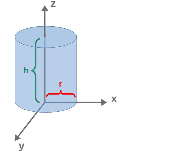
The cylinder here is centered at the origin.

To do this, we need to find appropriate integration limits for each of the coordinates x, y and z. The limits for z are easy; z just runs from 0 to h.

To find the limits for x and y, we can look at the x,y -plane (imagine looking at the cylinder from above), which just looks like a circle of radius r centered at the origin:

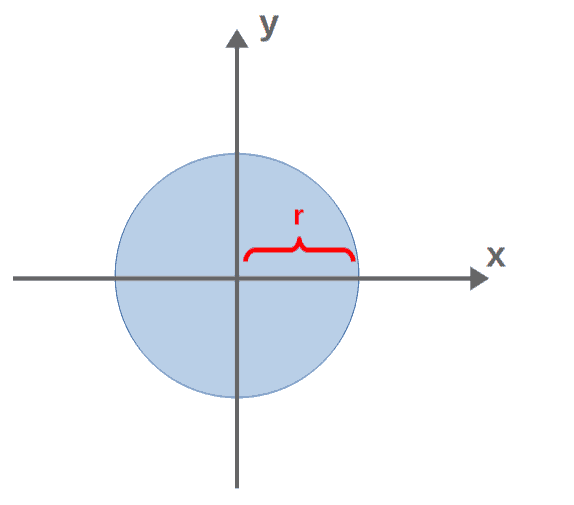
The limits of x therefore run from -r to r. As far as it comes to the limits of y, we can find these by solving the equation for a circle for y as a function of x:

x^2+y^2=r^2 Rightarrow y=pmsqrt{r^2-x^2}

We want our y to run through all of its values on the circle, so the integration limits for y will then be -√(r²-x²) and +√(r²-x²). So, our integration limits for the variables x, y and z are:

y=left[-sqrt{r^2-x^2}{,} sqrt{r^2-x^2}right]

We can now integrate our volume element, which will be:

V=int_V^{ }dV=int_0^hint_{-r}^rint_{-sqrt{r^2-x^2}}^{sqrt{r^2-x^2}}dydxdz — Note; I’ve chosen the order of integration such that we first integrate y, then x and then z. This is necessary, because the integration limits of y depend on the variable x, so we have to do the y-integral BEFORE the x-integral (since the result of the y-integral also gets integrated over x).

It’s easier to look at this integral in parts to avoid clutter. Let’s begin with the integral over y, which will give us:

int_{-sqrt{r^2-x^2}}^{sqrt{r^2-x^2}}dy=ybigg/_{!!!!!{-sqrt{r^2-x^2}}}^{sqrt{r^2-x^2}}=sqrt{r^2-x^2}-left(-sqrt{r^2-x^2}right)=2sqrt{r^2-x^2}

We then integrate this over x:

We can do a trig substitution here:

Doing this, dx will be:

The new limits of integration (the limits for which u runs over) can be obtained by looking at the relation x=rsin(u). For the lower bound (x=-r), u will be:

And for x=r, u will be:

Putting all of it together, the integral over x turns into:

int_{-r}^r2sqrt{r^2-x^2}dx Rightarrow 2int_{-frac{pi}{2}}^{frac{pi}{2}}sqrt{r^2-r^2sin^2u}rcos udu

We can simplify this a bit (by pulling out a factor of r from under the square root and then using 1-sin²u=cos²u)

2int_{-frac{pi}{2}}^{frac{pi}{2}}sqrt{r^2-r^2sin^2u}rcos udu=2r^2int_{-frac{pi}{2}}^{frac{pi}{2}}sqrt{1-sin^2u}cos udu=2r^2int_{-frac{pi}{2}}^{frac{pi}{2}}cos^2udu

This integral will give us just π/2:

2r^2int_{-frac{pi}{2}}^{frac{pi}{2}}cos^2udu=2r^2cdotfrac{pi}{2}=pi r^2

The last step is to integrate over the variable z:

int_0^hpi r^2dz=pi r^2zbigg/_{!!!!!0}^h=pi r^2h

So, all in all, the volume for our cylinder is:

That’s basically all there is to a multivariable integral (at least the key ideas) and this is enough for us to move forward with these concepts.

Now, it’s worth noting that many of the “integration tricks” from single-variable calculus still apply to multivariable calculus, but can be somewhat more complicated.

For example, the u-substitution method turns into something that generally requires the use of a Jacobian determinant (this is discussed in the lesson on coordinate transformations).

Lesson Summary

This lesson was fairly short, but here’s a quick summary of the key concepts:

Multivariable integrals are integrals over scalar fields (functions of multiple variables).
Multivariable integrals generally describe volumes of some sorts (whether that be an area, a 3D volume or a higher dimensional volume depends on the specific integral).
Multivariable integrals can usually be computed by simply integrating over each variable separately.

Vector Calculus For Physics: A Complete Self-Study Course

Curriculum