Line Integrals & Surface Integrals

In the last lesson, we discussed how curves and surfaces can be represented parametrically and how these representations can be used to calculate various geometric properties, such as arc length or surface area.

In this lesson, we’ll explore the concepts from the previous lesson more deeply by applying them to various types of integrals over both scalar and vector fields.

Then, the stuff you learn in this lesson can be directly applied to understand Stokes’ theorem and the divergence theorem, which will be topics of the next lesson.

A lot of the things in this lesson can be straightforwardly applied to physics and electromagnetism, such as in the form of Maxwell’s equations. We’ll look at some examples of this also to help you get some sense of what all of these concepts are useful for.

Lesson Contents

Line Integrals

The first concept we’ll look at is the notion of a line integral. A line integral essentially consists of two things; a scalar field or a vector field and a curve to integrate over.

So, in principle, a line integral is a way to integrate either a scalar field or a vector field over a particular curve.

Mathematically, we can compute these line integrals by parameterizing the curve (in fact, we also have to parameterize the field we’re integrating, but more on this soon), which we talked about in the previous lesson.

Anyway, we’ll begin by looking at line integrals of scalar fields as these are the simplest to understand.

Line Integral of a Scalar Field

A line integral of a scalar field essentially means taking a scalar field and integrating its values over some curve in 3D space.

As a reminder, in the last lesson, we calculated the arc length of a curve by integrating over all of the little “line elements”, ds, along the curve:

On the other hand, the line integral of a scalar field f(x,y,z) is defined as:

We can visualize what this line integral represents by looking at a two-variable scalar field f(x,y) and thinking of it as a surface with the height (the z-coordinate) being the value of the function at any given point.

The way to interpret the line integral is then as follows; we have a scalar field f(x,y) describing some “surface” and a curve γ that runs along the surface.

We then take the “height of the curve”, f(x,y), and multiply it by a small piece of arc length along the curve, ds. This gives us a small piece of area, dA, under the curve (you can think of f(x,y)ds as height*length, which gives some small area):

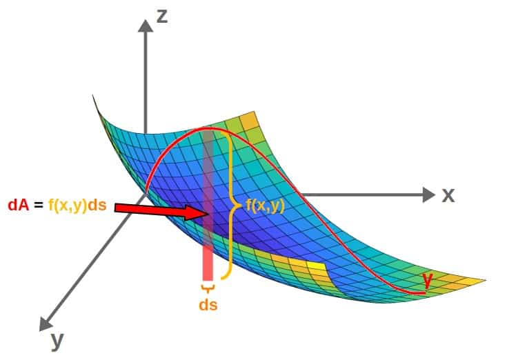
Then, adding up (i.e. integrating) all of these little pieces gives us the total area under this curve, which is the value of the line integral:

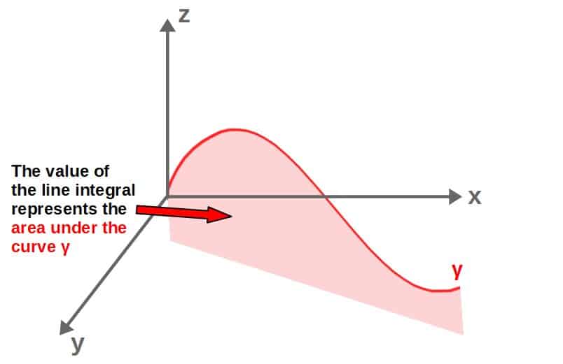
Therefore, the area under this curve is:

A=int_{gamma}^{ }fleft(x{,}y{,}zright)ds

Now, the question is; how do we calculate this line integral in practice?

Well, first of all, we need a parametric curve. In other words, we need the points (x,y,z) on the curve expressed in terms of a curve parameter t:

left(x{,}y{,}zright)=left(xleft(tright){,} yleft(tright){,} zleft(tright)right)

Using these, we parameterize the curve, but we also have to parameterize the scalar field we’re integrating.

In other words, we just write the scalar field in terms of the parameter t instead of x, y and z (by using the same parameterization as for the curve):

fleft(x{,}y{,}zright)=fleft(xleft(tright){,} yleft(tright){,} zleft(tright)right)=fleft(tright)

Also, remember from the last lesson where we concluded that the little “line element” ds can be written in terms of the magnitude of the parameterized tangent vector of the curve:

ds=left|frac{dvec rleft(tright)}{dt}right|dt

Therefore, the line integral or the area under the curve is then calculated as:

A=int_{gamma}^{ }fleft(x{,}y{,}zright)ds=int_a^bfleft(tright)left|frac{dvec{r}left(tright)}{dt}right|dt — Here, a and b are the end points of the curve γ.

Below is an example of calculating a line integral of a scalar field in the context of electromagnetism.

Physics Example: Calculating The Total Charge of a Non-Uniformly Charged Wire

An important physical application of the line integral of a scalar field is if we have a scalar field that describes, for example, an electric charge density along a curve (so charge per unit length).

Then, integrating along some curve, parameterized by t, (which could represent an electrically charged wire, in which the charge is distributed according to the charge density function) would give you the total charge of the curve or wire:

Q=int_a^blambdaleft(tright)left|frac{dvec{r}left(tright)}{dt}right|dt — It’s conventional to represent line charge density by the letter λ, which is why I’m using it here.

Let’s do a concrete example. Say we have an electrically charged wire that has the shape of a circle (a 2D curve) and the charge distribution along this wire is described by the charge density function λ(x,y):

lambdaleft(x{,}yright)=frac{lambda_0}{2pi r}left(x+frac{y^2}{2pi r}right) — Here, r is the radius of the circle and λ₀ is a constant with units of Coulombs/meter.

The goal is to calculate the total charge along the entire wire. Now, a circle (of radius r) can be expressed parametrically by the relations:

So, the position vector of any point on this wire (circle) is given by:

And the tangent vector is:

frac{dvec{r}left(tright)}{dt}=-rsin that{x}+rcos that{y}

Taking the magnitude of this, we get:

left|frac{dvec{r}left(tright)}{dt}right|=sqrt{r^2sin^2t+r^2cos^2t}=sqrt{r^2left(sin^2t+cos^2tright)}=r

Now, before we can integrate to find the total charge, we have to also express the charge density function in terms of the curve parameter t. This can be done by using the parametric relations x=rcos(t) and y=rsin(t):

lambdaleft(x{,}yright)=frac{lambda_0}{2pi r}left(x+frac{y^2}{2pi r}right) Rightarrow lambdaleft(tright)=frac{lambda_0}{2pi r}left(rcos t+frac{1}{2pi r}r^2sin^2tright)

Let’s simplify this a little bit by cancelling out some factors of r and using the relation sin²t=1-cos²t. Doing this, we get:

lambdaleft(tright)=frac{lambda_0}{2pi}left(cos t+frac{1}{2pi}-frac{1}{2pi}cos^2tright)

The total charge on the wire is then obtained by taking the line integral from 0 to 2π (which goes over the full circle):

Q=int_0^{2pi}lambdaleft(tright)left|frac{dvec{r}left(tright)}{dt}right|dt

Inserting the charge density function λ(t) and the magnitude of the tangent vector (which is just the constant r), we have:

Q=int_0^{2pi}frac{lambda_0}{2pi}left(cos t+frac{1}{2pi}-frac{1}{2pi}cos^2tright)rdt

Let’s pull out these constants and split the integral into three parts:

Q=frac{lambda_0r}{2pi}left(int_0^{2pi}cos tdt+frac{1}{2pi}int_0^{2pi}dt-frac{1}{2pi}int_0^{2pi}cos^2tdtright)

From the first integral, we get 0. From the second one, we get 2π and from the third one, we get just π (you can verify this by using, for example, the online integral calculator at Wolfram Alpha):

Q=frac{lambda_0r}{2pi}left(0+frac{1}{2pi}cdot2pi-frac{1}{2pi}cdotpiright)

So, the total charge on the wire is then:

Line Integral of a Vector Field

Instead of a scalar field, we can also take the line integral of a vector field. The only difference with this is that we now have a dot product inside of the integral:

int_{gamma}^{ }vec{F}left(x{,}y{,}zright)cdot dvec r

This dr-vector here essentially represent a small displacement along the curve. This vector is pointing in the direction of the curve (the same direction as the tangent vector).

If we have a parametric curve, the dr-vector can be calculated from the tangent vector:

dvec r=frac{dvec r}{dt}dt — Essentially, this little dr-vector is just an “infinitesimal version” of the tangent vector and in fact, the magnitude of this dr-vector is the little arc length line element ds (which you can see from taking the magnitude if this expression).

The line integral is then calculated as:

int_{gamma}^{ }vec{F}left(x{,}y{,}zright)cdot dvec{r}=int_a^bvec Fleft(tright)cdotfrac{dvec r}{dt}dt

Now, the right way to think about the line integral is that we “place” a curve in a vector field (similarly to how we “placed” a curve in a scalar field, which was represented as the height of some surface).

Then, at each point along the curve, we measure how much of that vector field is going along the curve. In other words, we can think of projecting the vector field onto the curve at each point. This is what the dot product is essentially doing.

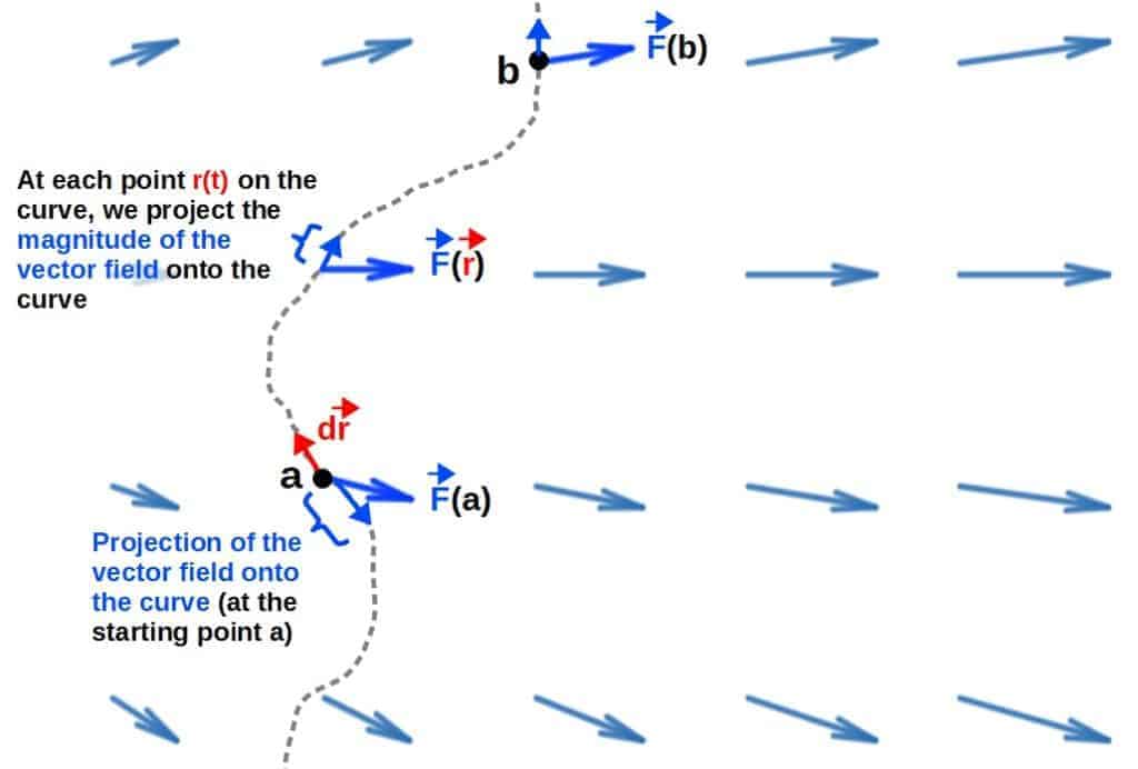
The blue vectors here represent the field vectors of the vector field F. You can imagine that the line integral gives you a number, which is basically the sum of the magnitudes of all these little “projection vectors” (F dotted with dr) at each point.

Then, the integral itself is basically adding up all of these projections of the vector field onto the curve, so in some sense, the line integral describes the “total amount” of the vector field F along the curve.

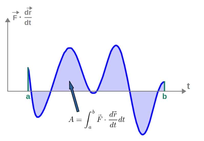
Another way to sort of visualize the value of the line integral is by imagining that we take the value of F*dr/dt at each and every point along the curve (which is a scalar field, so at each point, it gives you some number) and plot those values as a function of the curve parameter t.

The value of the line integral would then be the area under this curve:

Based on this visualization, both the scalar field line integral and the vector field line integral describe areas under a curve, in a sense.

Now, it’s a little difficult to give meaning to the value of the line integral in terms of mathematics only, but for example, in physics, the line integral of the force (which is generally a vector field) gives the work done by that force along some curve.

Sidenote: For certain types of vector fields, the value of the line integral only depends on the start and end points (and NOT the curve itself). These vector fields are called path-independent (or conservative vector fields in physics as these are used to describe forces that conserve energy) and in fact, any vector field that has zero curl is a path-independent vector field.

The explanation for this path-independence property comes from something called the gradient theorem and the fact that any vector field with zero curl can be written as the gradient of some scalar field. You'll explore this more in the problem set associated with this lesson.

Now, how do you calculate the line integral of a vector field in practice?

Well, you simply need a curve that is parameterized, but to do the actual integral, you also need to write the vector field in terms of the curve parameter.

Physics Example: Calculating The Work Done Along a Curve

Let’s say we have a force field (a vector field) that depends on x and y:

vec{F}left(x{,}yright)=kleft(-frac{xy}{l}hat{x}+xhat{y}right) — Here, k and l are constants with units of N/m and m.

We then want to calculate the work done by this force when some particle moves around a circle (from 0 to 2π). Now, a circle of a constant radius r can be parameterized by the relations:

Since we’re now talking about physics, we can imagine that the parameter t represents time. That’s why I’ve included this angular frequency, ω, here as it gives the correct units (note that this doesn’t change the shape of the curve at all).

So, as time increases, the particle moves around in a circular path, with its position given by the position vector:

vec{r}(t)=rcosomega that{x}+rsinomega that{y}

The tangent vector of the curve is given by the derivative of this:

frac{dvec{r}}{dt}=-romegasinomega that{x}+romegacosomega that{y}

Physically, this is the derivative of position with respect to time i.e. the velocity vector of the particle (as a function of time).

Now, before we do any integrals, we have to write the force field in terms of the parameter t (time) as well. This is quite simple; just plug in the relations x=rcos(ωt) and y=rsin(ωt) into the expression for the force to get the force on the particle as a function of time:

vec{F}left(tright)=kleft(-frac{xy}{l}hat{x}+xhat{y}right)=kleft(-frac{r^2}{l}sinomega tcosomega that{x}+rcosomega that{y}right)

We can now do the line integral to calculate the work by plugging the velocity vector and the force field into the integral and taking the dot product of these:

W=int_a^bvec{F}left(tright)cdotfrac{dvec{r}}{dt}dt=int_a^bkleft(-frac{r^2}{l}sinomega tcosomega tleft(-romegasinomega tright)+rcosomega tcdot romegacosomega tright)dt

Let’s simplify this to get:

W=kint_a^bleft(frac{r^3omega}{l}sin^2omega tcosomega t+r^2omegacos^2omegaright)dt

Now, before we go any further, let’s think about these integration limits a and b; we want to calculate the work done over a full circle. The time it takes for the particle to go one full cycle, T, can be calculated from the definition of the angular frequency:

omega=frac{2pi}{T} Rightarrow T=frac{2pi}{omega}

Therefore, our integration limits are a=0 and b=2π/ω. Our integral is then:

W=kint_0^{frac{2pi}{omega}}left(frac{r^3omega}{l}sin^2omega tcosomega t+r^2omegacos^2omegaright)dt

We can write sin²ωt as 1-cos²ωt (based on the identity sin²ωt+cos²ωt=1), so that we get:

W=kint_0^{frac{2pi}{omega}}left(frac{r^3omega}{l}left(1-cos^2omega tright)cosomega t+r^2omegacos^2omegaright)dt

=frac{kr^3omega}{l}int_0^{frac{2pi}{omega}}cosomega tdt-frac{kr^3omega}{l}int_0^{frac{2pi}{omega}}cos^3omega tdt+kr^2omegaint_0^{frac{2pi}{omega}}cos^2omega tdt — Here I’ve simply split the integral into three pieces.

The nice thing here is that the first two integrals are actually zero and the last integral gives us π/ω. Therefore, the work done by this force field around one loop is simply:

Now, as a sidenote, if we really think about the physics behind this, a non-zero work would mean that the particle’s speed (magnitude of the velocity vector) changes. However, in that case, we couldn’t describe it as the velocity vector given by:

Why? Because this actually has constant magnitude. Therefore, the net work done of all forces in this situation must be zero, so there must be an additional force involved in this situation that would cancel this work done by the force field we just calculated.

It would, in this case, be some sort of tension force (you can think of this as a string attached to the particle) that keeps the particle moving in a perfect circle. This tension force would then have to have a component along the curve that would cancel the work done by our force vector field defined earlier.

Circulation Integrals

An important special case of a line integral is a line integral around a closed curve or loop. This is called a circulation integral and we denote it as:

oint_{gamma}^{ }vec{F}left(x{,}y{,}zright)cdot dvec{r}

This is basically the same thing as an ordinary line integral, except that we’re doing the line integral over a closed curve. A closed curve is simply a curve that starts and ends at the same point.

In practice, calculating a circulation integral is exactly the same as calculating any line integral, the only thing is that the start and end points of the curve are the same:

oint_{gamma}^{ }vec{F}left(x{,}y{,}zright)cdot dvec{r}=int_a^avec Fleft(tright)cdotfrac{dvec{r}}{dt}dt

Now, you may want to ask; shouldn’t this integral always be zero since we’re integrating from t=a to t=a, which is basically an interval of zero? Well, it would be the case for ordinary integrals (such as ∫_a^a F(x)dx=0).

However, when integrating over a closed curve, we have to keep in mind that a closed curve is always periodic in a sense, meaning that two different values of the curve parameter can still correspond to the same point.

In fact, we saw an example of this earlier already when we did a line integral over a circle and got the following result:

int_0^{2pi}vec{F}left(tright)cdotfrac{dvec{r}}{dt}dt=pi r^2 — Here I’ve left out the constants we had in the “physics example”.

In reality, this is actually a circulation integral! This is because a circle is a closed curve with the “start” and “end” points, t=0 and t=2π, actually being the exact same point. Yet, we still got a non-zero result for the integral.

This is fundamentally explained by Stokes’ theorem, which actually tells us that for a vector field with non-zero curl, a closed line integral (circulation integral) will also generally have a non-zero value.

Therefore, the fact that a vector field may have a non-zero curl explains why a vector field may have some non-zero circulation value over a closed curve (I suppose this is where the name circulation comes from; the curl, in some sense, represents an infinitesimal notion of “circulation”).

Anyway, we’ll discuss these ideas more in the next lesson. For this lesson, we won’t need the notion of a circulation integral much.

Surface Integrals

A surface integral, just like a line integral, has to do with integrating either a scalar or a vector field. The difference here is that we’re now integrating along a surface instead of a curve.

Remember from the last lesson where we discussed how to parameterize a surface, calculate its normal vector and its surface area.

All of these concepts are applicable here also and if you learnt them well in the last lesson, the stuff we’ll discuss here shouldn’t be too difficult.

Surface Integral of a Scalar Field

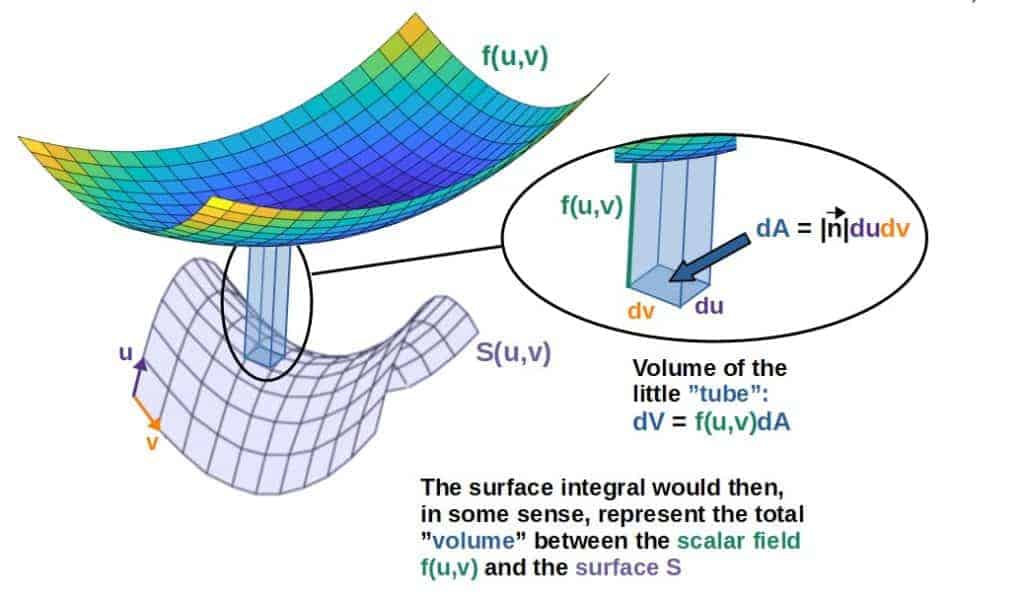
We’ll begin by discussing the surface integral of a scalar field. In the last lesson, we concluded that the surface area of a parametric surface S(u,v) can be calculated from the magnitude of the normal vector to the surface:

A=int_{ }^{ }int_S^{ }left|vec nright|dudv

Let’s now imagine that we have some scalar field f(x,y,z) and we want to integrate values of the scalar field along some parametric surface S(u,v).

Now, the first thing we have to do is express the scalar field in terms of the surface parameters, u and v, so f(x,y,z)=f(u,v). Once that’s done, well, we simply “add” the scalar field inside the integral as follows:

int_{ }^{ }int_S^{ }fleft(u{,}vright)left|vec{n}right|dudv

Now, the geometric idea behind what such an integral actually represents is a bit difficult to define precisely.

Essentially, as the scalar field produces some number at each point in space, we are, in a sense, adding up all of these numbers along the surface.

Now, the way you could imagine this is by picturing the scalar field as a surface with its “height” describing the value of the scalar field. The surface integral would then give you the volume between the surface and the scalar field:

In reality, you would actually be projecting the surface S onto the xy-plane, in which case this geometric picture would perhaps be more accurate.

Now, personally I don’t want to always picture such a geometry. Sometimes it’s just convenient to do a calculation without thinking of the geometry behind it too much.

In fact, sometimes we like to represent different things with these scalar fields, in which case this geometric notion doesn’t even make much sense.

For example, if the scalar field has some physical meaning, such as the electric charge density (charge per surface area). So, f(x,y,z) would give you the charge density at each point in space.

Then, by taking the surface integral of f(x,y,z), we would get the total charge on the surface. In this case, we’re not really thinking of any kind of volume, we’re going by a physical representation.

Down below, I’ve included an example of how to use these surface integrals in physics.

Physics Example: Calculating The Total Charge on a Cone Using Surface Integrals

This example goes as follows; we have a cone with its “curved sides” being electrically charged. The charge density on the surface is described by the function (scalar field):

sigmaleft(x{,}y{,}zright)=frac{sigma_0}{h^2}left(x^2-yzright) — Here, σ₀ is a constant with units of Coulombs/meter² and h is the height of the cone (a constant as well).

Now, the cone, as we deduced in the previous lesson, was parameterized (in terms of the surface parameters u and v) by:

x=ucos v{,} y=usin v{,} z=frac{h}{R}u — Here, h is again, the height of the cone and R is the radius of the bottom circle.

We also already calculated the magnitude of the normal vector in the last lesson, which was:

left|vec{n}right|=sqrt{h^2+R^2}frac{u}{R}

Before we can do the surface integral, we have to convert our charge density function into a function of u and v. This is done by simply plugging in the relations x=ucos(v), y=usin(v) and z=hu/R into σ(x,y,z):

sigmaleft(x{,}y{,}zright)=frac{sigma_0}{h^2}left(x^2-yzright) Rightarrow sigmaleft(u{,}vright)=frac{sigma_0}{h^2}left(u^2cos^2v-usin vcdotfrac{h}{R}uright)

So, our charge density function is then:

sigmaleft(u{,}vright)=frac{sigma_0}{h^2}left(cos^2v-frac{h}{R}sin vright)u^2

If we want to calculate the total charge on the surface of the cone, this can be done by taking the surface integral of this charge density function along the surface of the cone, which would be:

Q=int_{ }^{ }int_S^{ }sigmaleft(u{,}vright)left|vec{n}right|dudv

Plugging in the stuff we’ve obtained already, we have:

Q=int_{ }^{ }int_S^{ }frac{sigma_0}{h^2}left(cos^2v-frac{h}{R}sin vright)u^2sqrt{h^2+R^2}frac{u}{R}dudv

Now, the full surface of the cone runs from 0 to R (the limits of the parameter u) and 0 to 2π (limits of v). Therefore, this integral becomes:

Q=frac{sigma_0}{h^2R}sqrt{h^2+R^2}int_0^{2pi}left(cos^2v-frac{h}{R}sin vright)dvint_0^Ru^3du — Here I’ve pulled out the constants and separated the variables u and v.

From the u-integral, we get just R⁴/4. We can also split the v-integral into two:

Q=frac{sigma_0}{h^2R}sqrt{h^2+R^2}left(int_0^{2pi}cos^2vdv-frac{h}{R}int_0^{2pi}sin vdvright)frac{R^4}{4}

Now, the first integral gives us just π (without having to do the actual integral, which is somewhat tedious and not really the point of this example) and the second integral gives us zero. Therefore, we then have:

Q=frac{sigma_0}{h^2R}sqrt{h^2+R^2}left(pi-0right)frac{R^4}{4}=frac{sigma_0pi R^3}{4h^2}sqrt{h^2+R^2}

This is the total charge on the surface of the cone (the curved part of the surface). Hopefully from this, you can get some ideas of how these surface integrals are used in physics.

It’s worth mentioning that if we’re doing a surface integral in some well-known coordinate system, such as polar or spherical, it’s much easier to use something called the Jacobian determinant to write down the correct form of the integral in terms of the u- and v- parameters.

We’ll talk about this more in the lesson on coordinate transformations.

Surface Integral of a Vector Field (The Flux Integral)

Similarly to how we can take the line integral of a vector field along a curve, we can also take the surface integral of a vector field. However, this does not measure the vector field along the surface, but rather through the surface.

The surface integral of a vector field is calculated as:

int_{ }^{ }int_S^{ }vec{F}left(u{,}vright)cdotvec{n}dudv — Notice that once again, we have the vector field here expressed in terms of the surface parameter u and v. In other words, to calculate these integrals you always have to write down the vector field as F(u,v) instead of F(x,y,z).

Essentially, the surface integral of a vector field represents the amount of the vector field arrows passing through the surface. This is called the flux of the vector field.

We can visualize this by thinking about what the dot product here represents; the dot product between F and n tells you how much of the vector field (at any given point) is going in the direction of n.

Well, since n is the normal vector to the surface, this dot product also then represents how much of this vector field is passing through the surface at any given point:

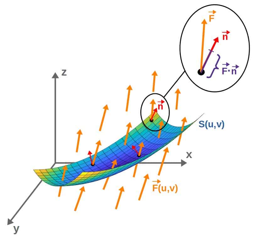
Then, when we take the integral, we essentially get the total amount of flux through the surface.

In terms of physical intuition, you could think of this vector field as the velocity of some fluid at each point. The surface integral of this velocity field would then give the total amount of fluid flowing through the surface (per unit time).

However, I want to stress again that the notion of the flux of a vector field does not necessarily have to have any physical meaning. It’s simply just a mathematical concept that CAN be given physical meaning, depending on the application.

Important sidenote: Given a surface and its normal vector, we basically have a choice of which "side" of the surface we take our normal vector pointing out of. In the example above, the normal vector is chosen to point upwards from the "top part" of the surface, but equivalently, we could take it to point downwards from the "bottom" of the surface. This is the problem of choosing an orientation for the surface.

This makes a difference when calculating dot products in these flux integrals; in particular, choosing the "oppositely pointing" normal vector will change the sign of the dot product (but not its actual value). The important thing is that you pick one orientation and stay consistent with it throughout the whole surface.

In practice, when you're calculating the normal vector using the cross product, you're free to choose either a plus or a minus sign. Both will work, but usually I'll just choose the positive choice.

Physics Example: Calculating The Mass of a Flowing Fluid Using Flux Integrals

Imagine a fluid in some 3D space that’s flowing around. Let’s now place a surface somewhere in this space and calculate the total mass of the fluid flowing through this surface in some period of time (in other words, we want to find the mass as a function of time).

The mass flux of a fluid is defined as the rate of change of the mass flowing through the surface per unit area:

vec{j}left(x{,}y{,}zright)=rhovec{v}left(x{,}y{,}zright) — Here ρ is the density of the fluid (assumed to be a constant) and v is the velocity of the fluid at each point in the space (a vector field).

If we integrate the mass flux over the surface area (i.e. flux integral), we then get the rate of change of the mass:

frac{dm}{dt}=int_{ }^{ }int_S^{ }vec{j}left(x{,}y{,}zright)cdotvec{n}dS=int_{ }^{ }int_S^{ }rhovec{v}left(x{,}y{,}zright)cdotvec{n}dS — Here, the dS=dudv, which is just a shorter way of writing the “surface area element”.

Now, expressed in terms of the surface parameter, this would be:

frac{dm}{dt}=rhoint_{ }^{ }int_S^{ }vec{v}left(u{,}vright)cdotvec{n}dudv

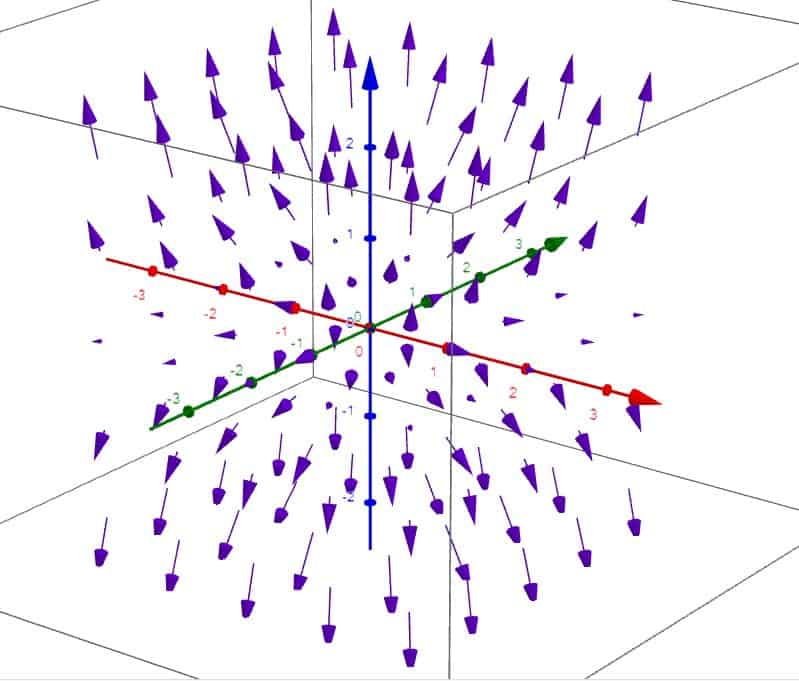
Let’s say we have a steady-state fluid (meaning that its velocity doesn’t vary with time, only with space) which has a velocity at each point (x,y,z) given by the vector field:

vec{v}left(x{,}y{,}zright)=v_0left(frac{kx}{x^2+y^2}hat{x}+frac{ky}{x^2+y^2}hat{y}+frac{z}{k}hat{z}right) — Here, v₀ has units of velocity and k (>0) has units of length.

This describes a “source” of outwards-flowing fluid centered at the origin:

Now let’s place a sphere of radius r at the center and calculate the flux through its surface. This will give us the rate of change of the mass of the fluid flowing through the surface of the sphere.

The first thing to do is to parameterize the surface of the sphere. This can be done using spherical coordinates, r, θ and φ, which are defined as:

x=rcosthetasinvarphi{,} y=rsinthetasinvarphi{,} z=rcosvarphi — With these spherical coordinates, θ runs from 0 to 2π and φ from 0 to π (for one “revolution” around the sphere).

Since the radius r here is a constant, the only variables we have are θ and φ, which I’ll rename to u and v just to keep consistent with our notation. We then have the coordinates x, y and z expressed in terms of u and v:

x=rcos usin v{,} y=rsin usin v{,} z=rcos v — Keep in mind for later the limits of these parameters; 0≤u≤2π and 0≤v≤π.

The position vector of a point on the surface of the sphere is then:

vec{r}left(u{,}vright)=rcos usin vhat{x}+rsin usin vhat{y}+rcos vhat{z}

Taking the partial derivatives of this, we get:

frac{partialvec{r}}{partial u}=-rsin usin vhat{x}+rcos usin vhat{y}+0hat{z}

frac{partialvec{r}}{partial v}=rcos ucos vhat{x}+rsin ucos vhat{y}-rsin vhat{z}

The components of the cross product between these two partial derivative vectors are:

left(frac{partialvec{r}}{partial u}timesfrac{partialvec{r}}{partial v}right)_x=rcos usin vcdotleft(-rsin vright)-0cdot rsin ucos v=-r^2cos usin^2v

left(frac{partialvec{r}}{partial u}timesfrac{partialvec{r}}{partial v}right)_y=0cdot rcos ucos v-left(-rsin usin vright)cdotleft(-rsin vright)=-r^2sin usin^2v

left(frac{partialvec{r}}{partial u}timesfrac{partialvec{r}}{partial v}right)_z=-rsin usin vcdot rsin ucos v-rcos usin vcdot rcos ucos v

=-r^2sin vcos vleft(sin^2u+cos^2uright)=-r^2sin vcos v

So, the normal vector to the sphere is (using these cross product components):

vec{n}=-r^2cos usin^2vhat{x}-r^2sin usin^2vhat{y}-r^2sin vcos vhat{z}

Now, since this has all minus signs, this is actually an inwards pointing normal vector. Equivalently, we can simply choose the normal vector opposite to this (which is still a normal vector to the sphere, it’s just pointing outwards from the surface), which has all plus signs:

There isn’t really any content with this choice, all it does is change the overall sign of the flux integral, which will now be positive for this choice of the normal vector orientation.

Anyway, before we calculate the flux integral, we have to also parameterize our velocity field in terms of u and v. Doing this, we get (by using the relations between x,y,z and u,v):

Rightarrow vec{v}left(u{,}vright)=v_0left(frac{krcos usin v}{r^2cos^2usin^2v+r^2sin^2usin^2v}hat{x}+frac{krsin usin v}{r^2cos^2usin^2v+r^2sin^2usin^2v}hat{y}+frac{rcos v}{k}hat{z}right)

This can be simplified a bit by using cos²u+sin²u=1 and cancelling some stuff, after which we have:

vec{v}left(u{,}vright)=v_0left(frac{kcos u}{rsin v}hat{x}+frac{ksin u}{rsin v}hat{y}+frac{rcos v}{k}hat{z}right)

Before we do the integral, let’s take the dot product between this velocity field and the normal vector:

vec{v}left(u{,}vright)cdotvec{n}=frac{v_0kcos u}{rsin v}cdot r^2cos usin^2v+frac{v_0ksin u}{rsin v}cdot r^2sin usin^2v+frac{v_0rcos v}{k}cdot r^2sin vcos v

=v_0krcos^2usin v+v_0krsin^2usin v+frac{v_0r^3}{k}cos^2vsin v

=v_0krsin v+frac{v_0r^3}{k}left(1-sin^2vright)sin v — To get to this step from the previous one, I factored out some stuff, used cos²u+sin²u=1 and cos²u=1-sin²u.

=left(v_0kr+frac{v_0r^3}{k}right)sin v-frac{v_0r^3}{k}sin^3v

That’s the dot product. We can now calculate the flux integral to give us the rate of change of mass:

Inserting the dot product we calculated and the integration limits (0≤u≤2π and 0≤v≤π), we get:

frac{dm}{dt}=rhoint_{v=0}^{v=pi}int_{u=0}^{u=2pi}left(left(v_0kr+frac{v_0r^3}{k}right)sin v-frac{v_0r^3}{k}sin^3vright)dudv

Since nothing in the integrand depends on u, we get just 2π from the u-integral:

frac{dm}{dt}=rhoint_{v=0}^{v=pi}left(left(v_0kr+frac{v_0r^3}{k}right)sin v-frac{v_0r^3}{k}sin^3vright)2pi dv

Moving some of these constants and splitting the integral into two, we get:

frac{dm}{dt}=2pirholeft(left(v_0kr+frac{v_0r^3}{k}right)int_{v=0}^{v=pi}sin vdv-frac{v_0r^3}{k}int_{v=0}^{v=pi}sin^3vdvright)

From the first integral, we get 2 and from the second integral, we get 4/3 (you can simply plug these integrals into a calculator, such as the online integral calculator at Wolfram Alpha). So, we have:

frac{dm}{dt}=2pirholeft(left(v_0kr+frac{v_0r^3}{k}right)cdot2-frac{v_0r^3}{k}cdotfrac{4}{3}right)

This can be simplified to the form:

frac{dm}{dt}=frac{4}{3}pirho v_0left(3kr+frac{r^3}{k}right)

This is the rate of change of the mass of the fluid flowing through the sphere’s surface. Now, this whole thing is just a constant, so we can simply integrate both sides to get:

int_{ }^{ }dm=frac{4}{3}pirho v_0left(3kr+frac{r^3}{k}right)int_{ }^{ }dt Rightarrow mleft(tright)=frac{4}{3}pirho v_0left(3kr+frac{r^3}{k}right)t+m_0 — This m₀ is an integration constant, which corresponds to the mass at t=0.

This is the mass of the fluid flowing through the surface of the sphere as a function of time. Now, hopefully this example illustrates the use of these flux integrals, especially in physics (and as a side benefit, we also parameterized the surface of a sphere and calculated its normal vector).

I want to also mention some alternative notation we’re going to be using for these surface integrals.

Some equations may become a little bit cluttered if we always carry around these u and v parameters in every integral. Instead, we can simply write the surface integral of a vector field as follows:

int_{ }^{ }int_S^{ }vec{F}left(u{,}vright)cdotvec{n}dudv Rightarrow int_{ }^{ }int_S^{ }vec{F}cdotvec{n}dS

Essentially, the only thing we’re doing is writing dudv=dS. You should, however, keep in mind that to actually calculate the surface integral, you have to still put back in this dudv-term. This is just a much nicer looking piece of notation.

Now, similarly to how we could take the line integral of a vector field over some closed curve, we can also take the surface integral of a vector field over a closed surface. We’re going to denote this as:

∯_Svec Fcdot vec ndS — Sometimes you’ll see this written in terms of a *unit* normal vector. However, this isn’t necessary if we’re defining dS as dudv.

So, essentially, this “circle” here just stands for the fact that we’re integrating over a closed surface. To actually calculate such a surface integral, well, it’s exactly the same as for a “non-closed” surface integral; calculate the normal vector to your surface, take the dot product, integrate over u and v etc.

In fact, we already saw an example of this above with the integral over the surface of a sphere, which of course, is a closed surface.

Now, the important thing about these closed surface integrals is that a closed surface always encloses some volume with the surface being the boundary of that volume. This turns out to be the key thing for understanding the divergence theorem.

Volume Integrals

I’m going to also briefly mention volume integrals, particularly for the reason that they are necessary for the divergence theorem, which will be discussed in the next lesson.

A volume integral of a scalar field essentially just means integrating the values of the scalar field over some volume. In particular, this gives you a triple integral:

I think the best intuition for this comes from physics; for example, the scalar field f here could represent a mass density function of a fluid (mass/volume), so this triple integral over a volume would then give the total mass of the fluid inside this volume.

As far as how to calculate these volume integrals, well, in Cartesian coordinates, this would simply be the triple integral over x, y and z that we’ve covered already in the lesson on multivariable integrals:

int_{ }^{ }int_{ }^{ }int_V^{ }fdV Rightarrow int_{ }^{ }int_{ }^{ }int_V^{ }fleft(x{,}y{,}zright)dxdydz — Notice that for these volume integrals, we don’t need to parameterize anything as this is just an ordinary triple integral. Moreover, there isn’t really a defined notion of a “parametric volume”.

Now, you can also do these triple integrals in other coordinate systems (such as spherical), but you’d have to convert them from Cartesian coordinates to that other coordinate system first using the Jacobian determinant (this will be covered in a later lesson).

In principle, you could also take the volume integral of a vector field, in which case, you’d get back another vector field (you would just be taking the volume integral of each of the components).

However, this is quite rarely used and we’re not going to need such a concept for any of the upcoming topics in this course.

Lesson Summary

There has been quite a bit of stuff covered in this lesson, but here are the key takeaways:

A line integral represents integrating something along a three dimensional curve (generally speaking).
We can take line integrals of both scalar and vector fields. The line integral of a vector field over a closed curve is called the circulation integral.
A surface integral represents integrating something over a surface embedded in a three dimensional space (generally).
Surface integrals can be taken of both scalar and vector fields. The surface integral of a vector field is called the flux integral.
Both line integrals and surface integrals generally require a parameterization of the curve or surface as well as expressing the scalar or vector field in terms of this parameterization.

Vector Calculus For Physics: A Complete Self-Study Course

Curriculum