Multivariable Calculus & Partial Derivatives

So far, we’ve only talked about how to take derivatives of functions that depend on one variable.

However, not all functions will always depend on only one variable, so differentiating these becomes a little more involved. This is what multivariable calculus is all about.

In this lesson, we’ll discuss various types of derivatives of scalar fields (multivariable functions). In later lessons, we’ll be discussing the same things but applied to vector fields (this is a little more complicated, generally speaking).

Lesson Contents

Multivariable Calculus: Why Do We Need It?

In physics, we often study quantities that may depend on multiple different variables.

For example, the electric field will generally be a vector field that is a function of both position (each of the coordinates x, y and z) as well as time in electrodynamics:

vec E=vec Eleft(x{,} y{,} z{,} tright) — Electric fields are also vector functions, to be accurate.

Now, say we wanted to differentiate the electric field (take a derivative of it). How would we do that since it depends on several different variables?

Well, the answer depends on what we’re interested in; if we wish to know how the electric field, or more generally, any scalar or vector field, changes with respect to only one of the variables, we need to use something called partial derivatives.

On the other hand, if we want to know how something changes in total (with respect to all of its variables), we need to use something called total derivatives.

Partial Derivatives

Let’s begin by discussing the idea of partial derivatives.

To put it simply, a partial derivative gives us a way to take the derivative of a multivariable function (that is, a function that may depend on multiple different variables) with respect to only one of the variables.

In other words, a partial derivative describes how a function of multiple variables changes as you change only one of its variables.

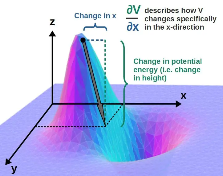
An example of this would be potential energy (V) in physics, which generally (in three dimensions) depends on all spacial coordinates (for example, the Cartesian coordinates x, y and z).

If we wish to know how the potential energy changes when we change only the x-variable, we simply take the partial derivative with respect to x (this actually gives you the x-component of force):

frac{partial V}{partial x}=F_x — Partial derivatives are denoted by the ∂-symbol (a “curly” d-letter).

So, this describes how the potential energy would change as we change the x-variable by a little bit. For example, imagine you’re on top of a hill and and your position is marked by some kind of Cartesian coordinate system. This partial derivative would describe the change in your potential energy in the x-direction as you move down the hill.

Imagine yourself moving down along this grey arrow. In general, you might move in the y and z directions also, but ∂V/∂x only gives the component of this change in potential in the x-direction. Respectively, ∂V/∂y would give the change in the y-direction and so on.

Now that we’ve established what partial derivatives are used for, the next question is; how do you actually use them in practice? How do you take a partial derivative of some function?

The answer is actually simple; you just treat all other variables as constant except the one you’re taking the partial derivative with respect to.

For example, if we have some function V(x,y)=x²+y², the partial derivative of this with respect to x would be ∂V/∂x=2x, since the derivative of a constant is zero, so the y-term goes to zero completely as we take its derivative (since y is treated as a constant).

Another Example of Taking Partial Derivatives

Let’s consider the function:

fleft(x{,}yright)=2xy^2+sinleft(xyright)

Let’s now take partial derivatives of this with respect to both x and y. First, the x-derivative:

frac{partial f}{partial x}=frac{partial}{partial x}2xy^2+frac{partial}{partial x}sinleft(xyright)

Since we’re treating y as a constant, it remains untouched from the first term (the derivative of 2*constant*x is just 2*constant). So, from that we have:

frac{partial}{partial x}2xy^2=2y^2 — If you wanted to, you could just think of 2y² here as simply a constant coefficient on x, which can be moved outside the derivative.

The second term will require the chain rule, which we talked about in the last lesson. So, first we differentiate the sin-part without worrying about what’s inside its argument. The derivative of sine will just give cosine.

Now, we also have to multiply by what’s inside the argument, namely by the partial derivative of xy:

frac{partial}{partial x}sinleft(xyright)=cosleft(xyright)cdotfrac{partial}{partial x}xy

Here, y is just a constant again, so we just get y from this derivative (a common mistake here would be to forget that you’re treating y as a constant and start using the product rule or something; this, however, would not be correct!):

cosleft(xyright)cdotfrac{partial}{partial x}xy=ycosleft(xyright)

Putting it all together, we have the partial derivative of f with respect to x:

frac{partial f}{partial x}=2y^2+ycosleft(xyright)

Now, let’s do the same but with respect to y:

frac{partial f}{partial y}=frac{partial}{partial y}2xy^2+frac{partial}{partial y}sinleft(xyright)

The process is exactly the same, but now we’re treating y as our variable and x is simply a constant. From the first term, we get:

frac{partial}{partial y}2xy^2=2xcdot2y=4xy

From the second term, we again have to use the chain rule:

frac{partial}{partial y}sinleft(xyright)=cosleft(xyright)cdotfrac{partial}{partial y}xy=xcosleft(xyright)

All in all, we have that the partial derivatives of this function are:

frac{partial f}{partial y}=4xy+xcosleft(xyright)

Some Partial Derivative Notation

Partial derivatives actually have quite many different notational conventions used for them. Here I’ll go over some of the most common ones, so you’ll be able to recognize them in the future.

The most common notation and also the most explicit, of course, is the one we’ve been using so far:

$frac{partial f}{partial x}$

Sometimes you’ll see this written as simply:

This notation is especially common in, for example, general relativity (such as in the Einstein field equations), where this use of index notation is quite common.

Some people also write this as:

So, this notation uses a subscript to denote differentiation with respect to some variable. Personally, I’m not a huge fan of this notation as it may be confusing when dealing with vector fields (f_x could also denote the x-component of the vector field f).

In this course, moving forward I’ll be using the regular explicit notation for partial derivatives, namely ∂f/∂x.

Second & Mixed Partial Derivatives

Another worthwhile concept to discuss is the second partial derivative.

Just like ordinary second derivatives, we can also take second partial derivatives, which just means we’re differentiating the function twice with respect to some variable. The notation for this is the same as for ordinary second derivatives:

$frac{partial^2f}{partial x^2}$

Now, something that’s also possible with a partial derivative is the notion of mixed partial derivatives. Let’s say we were to take the y-derivative of the x-derivative of a function:

frac{partial}{partial y}frac{partial f}{partial x}

In general, this is a second derivative, but with each of the derivatives taken with respect to different variables. A commonly used notation for this is:

frac{partial}{partial y}frac{partial f}{partial x}=frac{partial^2f}{partial ypartial x}

It’s also worth noting that the the order in which you take these mixed derivatives typically does not matter. In other words:

frac{partial^2f}{partial ypartial x}=frac{partial^2f}{partial xpartial y}

There are some exceptions to this, however, if f is what physicists usually call a “well-behaved function”, then the order of partial derivatives generally won’t matter. This is most often the case in physics.

Total Derivatives

Partial derivatives measure the change in a function as we change one of its variables. However, what if we wanted to know how a function changes with respect to all of its variables.

This is where the total derivative comes in.

Now, let’s say we want to know how a function f(x,y) changes with respect to some other variable t.

This may seem weird since f does not explicitly depend on t, however, the coordinates or variables x and y might depend on t. If they do, we can take the total derivative of f with respect to t.

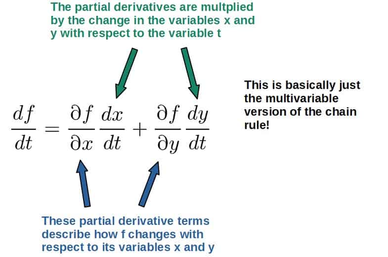
The total derivative of a function f(x,y) with respect to t is defined as follows:

If you’re wondering why we use the same notation (df/dt) for the total derivative as we do with the “ordinary” derivative, this is because *they are the same*; an ordinary derivative is really a total derivative, but in the case of single-variable functions, it doesn’t require the use of these partial derivatives.

Now, if this seems overwhelming, let’s look at a simple physical example. Say our function f is the potential energy function V(x,y) in two dimensions (potential energy generally depends spacial position, i.e. the x,y -coordinates in a Cartesian system).

Then, if we want to know how the potential energy changes in total with time, we simply take the total derivative with respect to time (just replace f with V in the above formula):

frac{dV}{dt}=frac{partial V}{partial x}frac{dx}{dt}+frac{partial V}{partial y}frac{dy}{dt}

Now, these time derivatives (dx/dt and dy/dt) are simply the components of velocity in the x- and y -directions, respectively (so, dx/dt=v_x and dy/dt=v_y).

Moreover, we define these partial derivatives of the potential as the negative components of force (the conservative force that results from the change in this potential).

So, this becomes:

frac{dV}{dt}=-F_xv_x-F_yv_y=-left(F_xv_x+F_yv_yright)

Now, what is this thing? It’s the sum of the products of vector components, which is just the dot product between the F and v vectors. All in all, this becomes:

This equation describes the rate of change of the potential energy V of an object moving with velocity v under the (conservative) force F.

A Comparison of Partial vs. Total Derivatives Through An Example

It may be instructive to compare partial derivatives and total derivatives to one another and see what we can learn. In particular, we’ll do this through an example.

Consider, for example, the function:

Now, when we usually think of functions, we typically consider y as a function of x, i.e. y=y(x). Let’s also assume this here, so that what we have here is actually y as an implicit function of x.

When taking partial derivatives, this does not matter since partial derivatives are not concerned whether something is an implicit function of something else. We simply just take the derivative only whenever there is an explicit term with that variable. So, the partial derivative of f with respect to x is then:

However, if we take a total derivative with respect to x instead, it does indeed matter that y depends on x. Let’s see how exactly. So, we just use the formula for total derivatives (from the formula from earlier, just replace t with x). We then have:

frac{df}{dx}=frac{partial f}{partial x}frac{dx}{dx}+frac{partial f}{partial y}frac{dy}{dx}=frac{partial f}{partial x}+frac{partial f}{partial y}frac{dy}{dx} — Here I’ve used the fact that dx/dx=1.

From the first term, we have:

frac{partial f}{partial x}=frac{partial}{partial x}x^2y^2=2xy^2

From the second term, we get:

frac{partial f}{partial y}frac{dy}{dx}=frac{partial}{partial y}x^2y^2frac{dy}{dx}=2x^2yfrac{dy}{dx} — Since we don’t know how y actually depends on x, we’ll just leave this dy/dx -term as it is.

Therefore, the total derivative df/dx is then:

Let’s now compare this to the partial derivative with respect to x:

We can clearly see that the total derivative has an additional term with dy/dx, which comes from the fact that y implicitly depends on x. If it didn’t and y was just an independent variable, this term would be zero.

Hopefully you can see the meaning of the total derivative here; a total derivative also accounts for any dependence that the variables x and y may have on one another. Thus, in addition to giving the change in f as we change x, the total derivative also gives the change in f caused by the change in y since x changes (since y is a function of x).

In contrast, the partial derivative only describes the change in f directly as x changes, but does not account for the fact that y also changes with x.

The Total Differential

Another useful concept directly related to the total derivative is the total differential. To introduce this, let’s look at the total derivative of a function f(x,y) with respect to a variable t again:

frac{df}{dt}=frac{partial f}{partial x}frac{dx}{dt}+frac{partial f}{partial y}frac{dy}{dt}

Now, since each term has a dt in the denominator, we can “cancel” out each of them (this is sort of a lose way of doing it mathematically, since these are technically operators, however, this can be proven to “work” in a rigorous way as well):

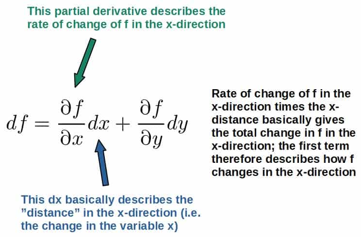
df=frac{partial f}{partial x}dx+frac{partial f}{partial y}dy

Here we basically have the change in a function caused by a change in each of its variables. This is called the total differential of f.

The difference between this and the total derivative is that the total derivative describes the total change in f caused by a change in some particular variable.

The total differential, on the other hand, describes the total change in f due to a change in all of its variables.

Intuitively, the total differential actually has a quite simple interpretation. What we basically have on the right hand side are the rates of change of f in each coordinate direction multiplied by the “distances” in each direction:

Lesson Summary

In this lesson, we somewhat briefly went over the necessary concepts we’re going to need when dealing with vector fields and vector calculus.

The most important points you should take away from this lesson are:

Multivariable calculus is used to describe how a function of several variables changes. In other words, it has to do with differentiating scalar fields.
A partial derivative describes the change in a multivariable function with respect to one of its variables.
A total derivative is used to describe the total change in a function with respect to some implicit variable.
A total differential is used to describe the total change in a function caused by a change in all of its variables.

Vector Calculus For Physics: A Complete Self-Study Course