Parametric Curves & Surfaces

In this lesson, we’ll be discussing some important geometric constructs that come up in vector calculus, namely, various kinds of curves and surfaces.

We’ll also discuss how these curves and surfaces are describes parametrically and how this, on the other hand, can be used to calculate various different things.

In the next lesson, we’ll be taking a closer look at different mathematical procedures that use the concepts discussed here, such as line integrals and surface integrals.

Lesson Contents

What Are Curves & Surfaces?

To begin discussing the notions of curves and surfaces and everything associated with these, we need to establish some notation and some conventions I’m going to be using.

So far, we’re familiar with the notion of a curve in two dimensions, such as in the xy-plane. This is simply a collection of specific points that forms some kind of a curve-like shape:

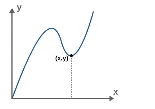
You can think of this as a function with an input (in this case, x) that outputs a point for each input.

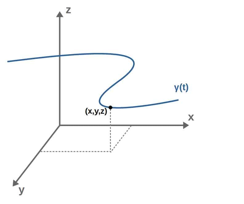
Similarly, we can have a curve in three dimensions, which you can think of as a function (I’ll denote this as γ(t)) that takes an input (the curve parameter t, which we’ll discuss later) and outputs, in this case, three values corresponding to the point (x,y,z) on the curve:

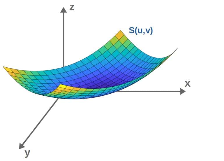
A surface in 3D, on the other hand is, we’ll, what you might expect; a surface in 3D:

The distinction between a curve and a surface is that a surface is parameterized by two parameters (u,v) and a curve with only one (t). So, while a curve only describes one point for each value of t, a surface can describe multiple points for one value of u, for example. In other words, a single point on the surface requires two distinct parameters.

In this lesson, we’re going to discuss everything you need about curves and surfaces to then be able to do, for example, surface and line integrals of vector fields in the upcoming lessons (and ultimately, to be able to understand Stokes’ and divergence theorems).

Describing Curves Parametrically

To describe a curve γ, we need a parameterization for the curve. To get such a thing, we choose some suitable curve parameter, t. We’ll then denote the parameterized curve as γ(t), though this is just notation and nothing too important.

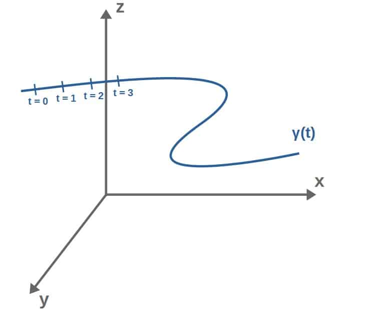
You can kind of visualize the curve parameter t by imagining that you place a “coordinate axis” or tickmarks that describe points along the curve:

This form of parameterization of “tickmarks” along the curve is called the arc length parameterization, however, it’s worth noting that we can choose other types of parameterizations as well (such as an angle relative to some axis). So, this is just one way to visualize a parametric curve.

Now, we’re not necessarily interested in the values of this curve parameter t, rather the whole point of this parameter is to be able to express points on the curve (x,y,z) in terms of this parameter.

To do this, we simply write the points (x,y,z) along the curve as functions of this parameter, so x(t), y(t), z(t).

A neat little way to express these points is by imagining a little position vector that points from the origin to a point (x(t),y(t),z(t)) on the curve:

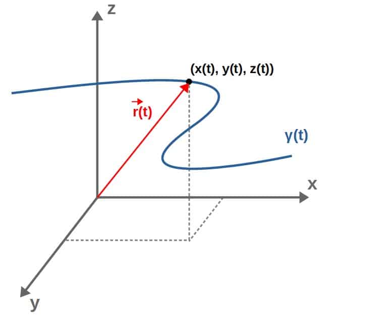
The components of this position vector are then simply the points on the curve expressed through the curve parameter t, so we can write it as:

vec{r}left(tright)=xleft(tright)hat{x}+yleft(tright)hat{y}+zleft(tright)hat{z}

Let’s look at a little example to better understand how this really works in practice. We can imagine a curve as having the following parameterization:

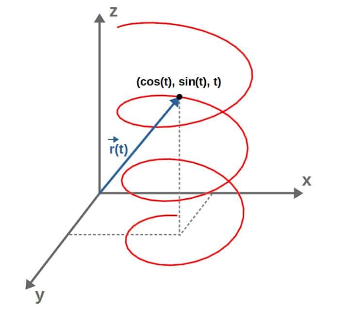
These give the coordinates of any point on the curve. The position vector of any point on this curve is therefore:

vec{r}left(tright)=cos that{x}+sin that{y}+that{z}

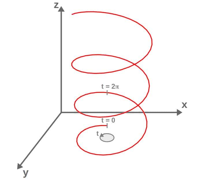
This particular curve happens to describe a spiral-like curve that essentially that does circles in the xy-plane and at the same time, increases linearly in the z-direction:

So, that’s essentially all there is to describing curves parametrically. Next, we’ll look at what to actually do with these parametric curves and how we can use them in practice.

Finding The Tangent Vector To a Curve

An important concept associated with curves is the tangent vector of a curve. The tangent vector is calculated by differentiating the position vector with respect to its parameter t:

frac{dvec{r}left(tright)}{dt}=frac{dxleft(tright)}{dt}hat{x}+frac{dyleft(tright)}{dt}hat{y}+frac{dzleft(tright)}{dt}hat{z}

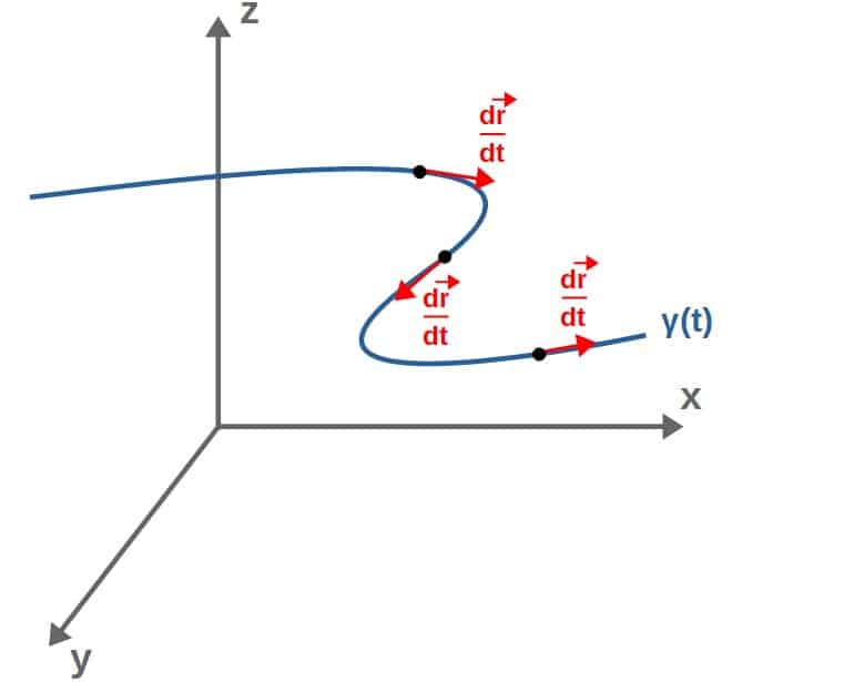
Now, this is called a tangent vector because it lies tangentially to the curve at each point (this is because the derivative generally describes tangents to curves, like you may have seen in single-variable calculus with the “slope of a tangent line”).

In other words, the tangent vector always points in the direction that the curve is going in:

The magnitude of this tangent vector describes the rate of change of the coordinates along the curve with respect to the curve parameter. In practice, this can be calculated just like the magnitude of any vector:

left|frac{dvec{r}}{dt}right|=sqrt{left(frac{dx}{dt}right)^2+left(frac{dy}{dt}right)^2+left(frac{dz}{dt}right)^2}

So, to recap, the tangent vector to a curve is a vector that points in the direction of the curve at each point and its magnitude describes how fast the coordinates are changing along the curve.

As an example, let’s consider again the spiral curve from before, which was described by the position vector:

The tangent vector to this curve is:

frac{dvec{r}}{dt}=-sin that{x}+cos that{y}+hat z

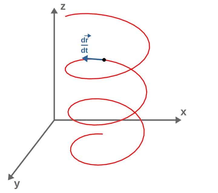
We can also take the magnitude of the rate of change, which describes how fast the coordinates are changing along the curve, which gives us:

left|frac{dvec{r}}{dt}right|=sqrt{sin^2t+cos^2t+1}=sqrt{2} — Here, i’ve used the fact that sin²t+cos²t=1.

So, for this curve, we get a tangent vector with a constant magnitude.

This essentially means that as we move along the curve, the coordinates increase with a constant rate of change.

A nice way to think of this is by imagining that this curve describes the trajectory of a particle, in which case the particle would move with a constant speed.

In fact, a charged particle in a constant magnetic field will move exactly along such a curve described above and its speed will remain constant because physically, a magnetic field doesn’t do any work.

Computing The Arc Length of a Curve

An important application of the tangent vector explained above is for computing the arc length of a curve. Essentially, the arc length (Δs) is the length of a “piece” of the curve:

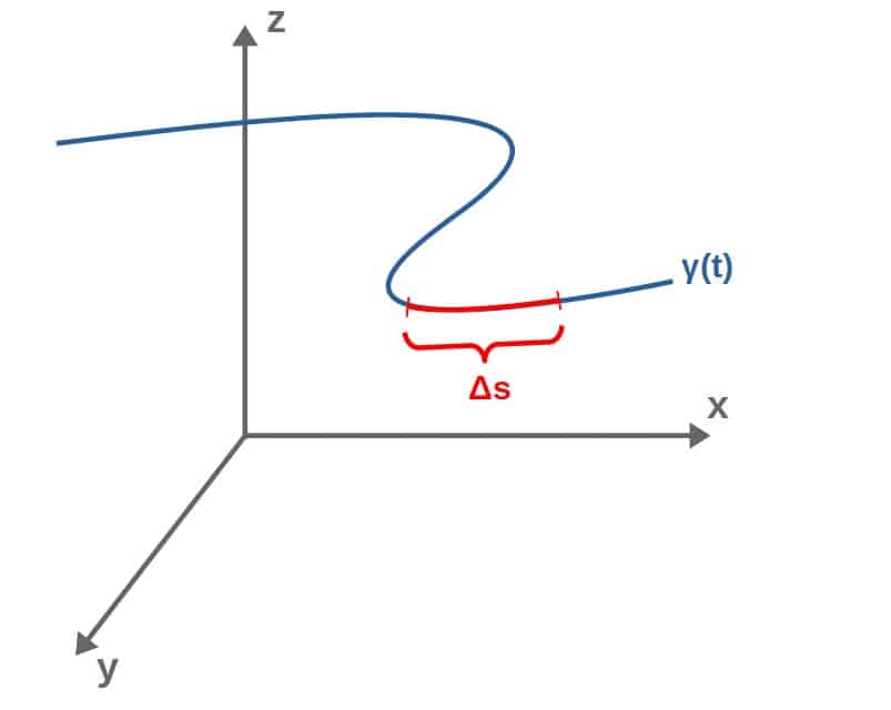
To calculate the total arc length, we can imagine that we “split” this arc into multiple little pieces with length ds:

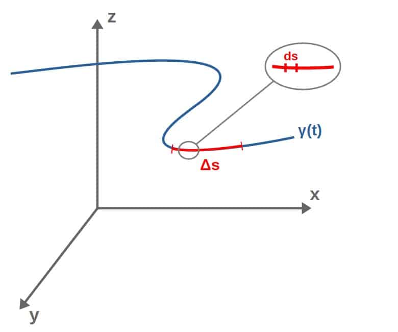
The length ds of each little piece can then be calculated as the rate of change (magnitude of the tangent vector), dr/dt, at that point multiplied by the change in the curve parameter, dt. You can think of this as distance=velocity*time, i.e. dx=dx/dt*dt.

Now, this works if we imagine that the piece ds is small enough (infinitesimal, to be exact) so that the rate of change is basically constant along that little ds.

Anyway, the length of each piece ds is then:

Then, the total arc length, Δs, of the segment we’re interested in is obtained by integrating all of these ds-pieces:

Delta s=int_a^bds=int_a^bleft|frac{dvec{r}left(tright)}{dt}right|dt — Here, a and b are the start and end points of the arc segment we’re integrating over.

As an example, let’s calculate the arc length of the spiral curve we had earlier. I’ll choose the start and end points as 0 and 2π.

Now, since in our position vector for the curve, the parameter t is contained in both the trigonometric terms (cos(t) and sin(t)) describing circular “motion” and also in the linear term, we can imagine that it characterizes both a “height” and an “angle” (see the picture below).

Anyway, doing the actual arc length calculation, we get:

Delta s=int_0^{2pi}left|frac{dvec{r}}{dt}right|dt=int_0^{2pi}sqrt{2}dt=2pisqrt{2} — Reminder; the magnitude of the tangent vector is √2 (from earlier).

Now, just to recap, the steps to parameterize a curve and calculate its arc length is as follows:

Choose a suitable parameterization that expressed the coordinates of each point along the curve as functions of the curve parameter t. So, x=x(t), y=y(t) and z=z(t).
Write down the position vector as a function of the curve parameter t by using the coordinate expressions from step #1.
Calculate the tangent vector to the curve by differentiating the position vector.
Calculate the arc length by integrating the magnitude of the tangent vector.

Describing Surfaces Parametrically

In a similar manner as we described curves parametrically, we can also do the same for a surface. The only difference here is that we need two parameters to describe a point on the surface. I’ll call these surface parameters u and v.

But why two parameters? Well, a surface is basically a “piece of area” and areas always require two dimensions to describe them.

You could visualize the situation by imagining that there is a “coordinate grid” placed on the surface. Then, there are basically two independent directions you can move in, so you need two parameters to know which point on the surface you move to.

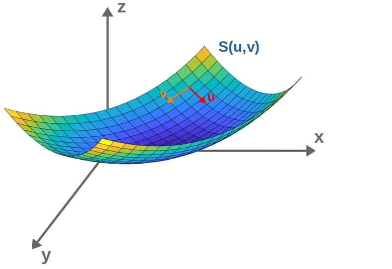
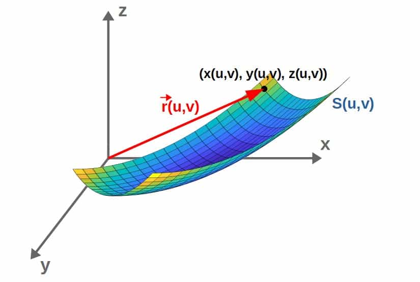
Visualization of the two surface parameters. Note that when we parameterize a surface, we aren’t *literally* placing a “coordinate system” on the surface, but rather, the parameterization is mostly a mathematical tool that often does not have a neat intuitive meaning.

Using the surface parameters, we can describe any point (x,y,z) ON the surface by writing down the coordinates as functions of the curve parameters in some suitable way (generally, there are more than one “correct” way to choose the parameterization):

x=xleft(u{,}vright){,} y=yleft(u{,}vright){,} z=zleft(u{,}vright)

Then, similarly to what we did for a curve, we can form a position vector that points from the origin to a point (x,y,z) on the surface. This position vector will then be a function of the surface parameters u and v:

vec{r}left(u{,}vright)=xleft(u{,}vright)hat{x}+yleft(u{,}vright)hat{y}+zleft(u{,}vright)hat{z}

As a sidenote, you may see a pattern with these parameterizations; we're taking a geometry that essentially requires three variables to describe (the coordinates x, y and z) and reducing it to require less variables (in the case of a curve, only one variable, the curve parameter t and for a surface, two variables u and v), but still describing the exact same thing. Therefore, in many ways, this process of parameterization makes everything simpler and it also allows us to directly calculate properties of the geometry we're describing.

Example: Parameterizing a Cone

Let’s do a little example of parameterizing a cone (with total height h and radius of the “bottom circle” R) that is centered at the origin of the xy-plane:

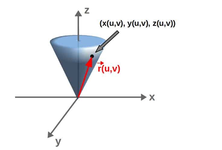
So, we want to find the position vector by finding a parameterization, u and v, for each of the coordinates x, y and z. First of all, if we look the the cone from above, it forms a circle of radius r in the xy-plane:

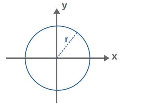
We can parameterize a circle using the polar coordinate relations x=rcosθ and y=rsinθ. Now, to keep consistent with our u,v-notation, I’ll simply relabel r to u and θ to v. So, we then have the parameterization for x and y:

Now, to find the parameterization of z, we can draw a little picture here:

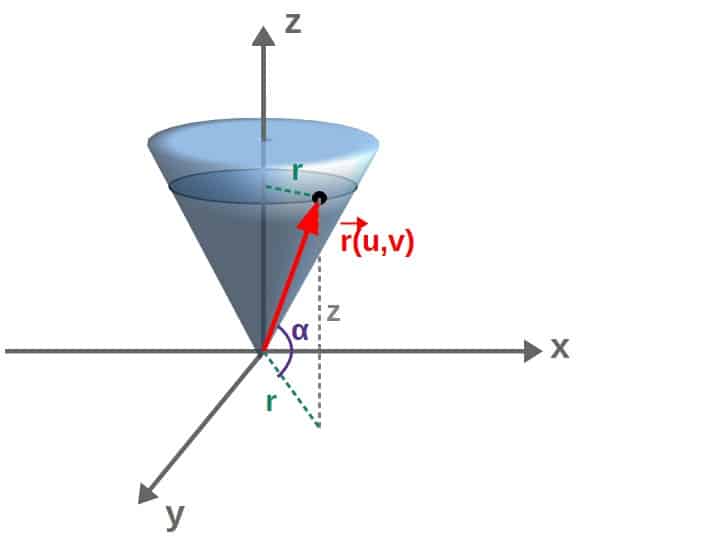
So, at any point on the surface of the cone, the “height” of that point is z. We can find z by looking at the angle α, which based on the picture, can be calculated as (using basic trigonometry):

However, the angle α is constant since it’s the angle between the cone and the x-axis. Therefore, we can also obtain the angle by looking at the “full” cone:

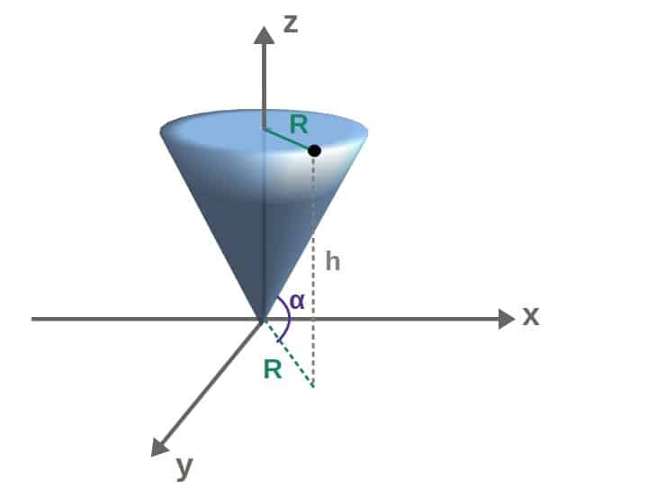
The angle here is the exact same angle α as in the last picture (can you see why?), so we can also calculate it as:

We can then relate this and the expression for tanα from earlier to get:

tanalpha=frac{z}{r}=frac{h}{R} Rightarrow z=frac{h}{R}r

Again, to keep consistent with our notation, we’ll set r=u. Therefore, our parameterization for the cone is:

Using these, the position vector of any point on the surface of the cone can then be written as:

vec{r}left(u{,}vright)=ucos vhat{x}+usin vhat{y}+frac{h}{R}uhat{z}

That’s the full parameterization of the cone! Note, however, that the limits of these parameters are 0≤u≤R (u represents the radius of the “bottom circle”) and 0≤v≤2π (v represents the angle around the circle). We will use these limits when we get to integrating the surface area of this cone.

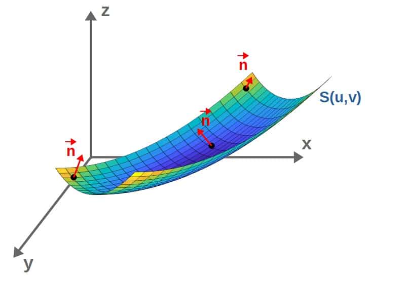
Finding The Normal Vector To a Surface

A normal vector to a surface is a vector that is perpendicular to the surface at any point on the surface. I’ll represent the normal vector of a surface by n (and if it’s a unit normal vector, I’ll put a hat on top of it).

Now, we want to find normal vectors to surfaces, because it turns out that this is how we can calculate the surface area of any parametric surface. In addition, we can also use these normal vectors later when we get to flux integrals, for example.

In practice, the normal vector of a surface parameterized by u and v can be computed by:

vec{n}=frac{partialvec{r}left(u{,}vright)}{partial u}timesfrac{partialvec{r}left(u{,}vright)}{partial v} — If you want to make this a unit normal vector simply divide this expression by the magnitude of the vector n.

Let’s think about why this gives us a normal vector.

First of all, the partial derivatives of r with respect to u and v give us vectors that point in the directions of u and v, respectively (for example, differentiating r with respect to u results in a vector that points in the direction of u).

Together, these partial derivative vectors, at each point on the surface, form a parallellogram of some sorts (see the picture below).

Then, taking the cross product of these two partial derivative vectors gives us a vector that is perpendicular to both of them. Or in other words, perpendicular to the parallellogram formed by the partial derivative vectors and therefore, also perpendicular to the surface itself.

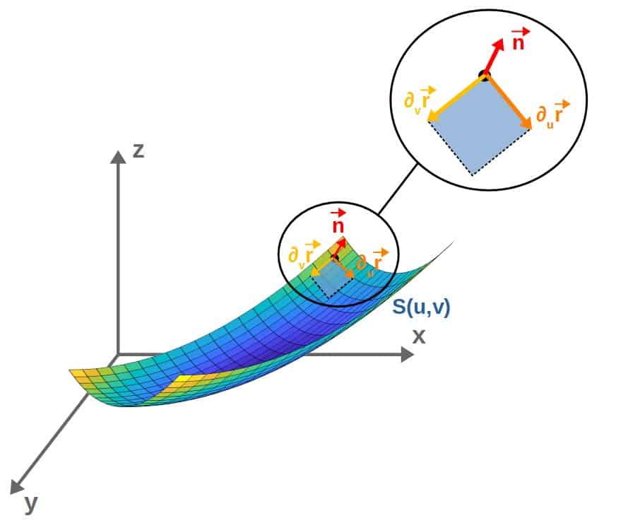
So, to put it simply, you get a normal vector by taking the partial derivatives of the position vector both with respect to u and v and then take the cross product of those vectors (to be precise, this gives you a vector field with vectors perpendicular to the surface at each point).

Example: Normal Vector To a Cone

Let’s calculate the normal vector to the cone we parameterized in the last example. As a reminder, the u,v-parameterized position vector we found for the cone was:

We’ll begin by calculating the partial derivatives of this position vector, both with respect to u and v:

frac{partialvec{r}}{partial u}=cos vhat{x}+sin vhat{y}+frac{h}{R}hat{z}

frac{partialvec{r}}{partial v}=-usin vhat{x}+ucos vhat{y}+0hat{z}

Now, let’s take the cross product of these two vectors. We’ll do each component separately. First, for the x-component of the cross product, we have:

left(frac{partialvec{r}}{partial u}timesfrac{partialvec{r}}{partial v}right)_x=sin vcdot0-frac{h}{R}cdot ucos v=-frac{h}{R}ucos v

Then, for the y-component, we get:

left(frac{partialvec{r}}{partial u}timesfrac{partialvec{r}}{partial v}right)_y=frac{h}{R}cdotleft(-usin vright)-cos vcdot0=-frac{h}{R}usin v

And last, the z-component:

left(frac{partialvec{r}}{partial u}timesfrac{partialvec{r}}{partial v}right)_z=cos vcdot ucos v-sin vcdotleft(-usin vright)=ucos^2v+usin^2v=u

We can then form the full cross product vector from these components:

frac{partialvec{r}}{partial u}timesfrac{partialvec{r}}{partial v}=-frac{h}{R}ucos vhat{x}-frac{h}{R}usin vhat{y}+uhat z

This is then also our normal vector (i.e. the vector field that is perpendicular to the surface at every point):

vec{n}=-frac{h}{R}ucos vhat{x}-frac{h}{R}usin vhat{y}+uhat{z}

Now, the next question is; what do we actually do with this normal vector? Well, one important application is for calculating the surface area of any parametric surface, so let’s look at this next.

Computing Surface Area of a Parametric Surface

To calculate the surface area of a parametric surface, we can use similar logic as we did for the normal vector.

In fact, let’s do the exact same calculation but with a small twist; instead of the partial derivative vectors, we can look at the (small) changes in the position vector in each of the u- and v-directions separately:

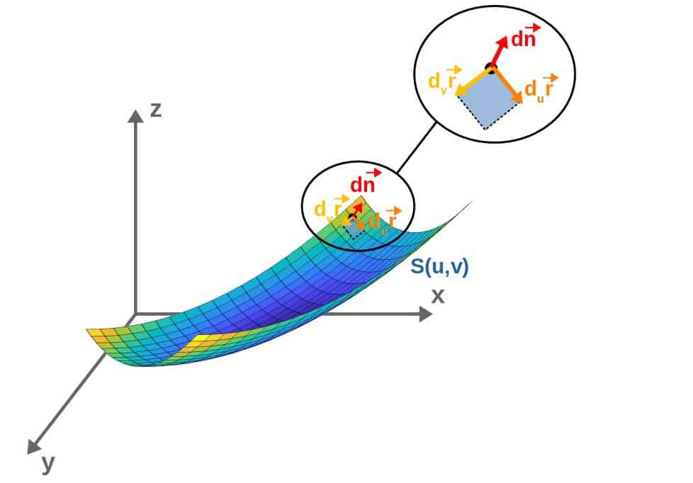
Here, d_vr and d_ur are the changes in the vector r in the directions of u and v. The only difference here to the calculation we did before is that d_vr and d_ur give us vectors that are *infinitesimally* “short”. Therefore, also the normal vector, dn, resulting from these is going to be “infinitesimally short”.

We can calculate the normal vector dn again as a cross product:

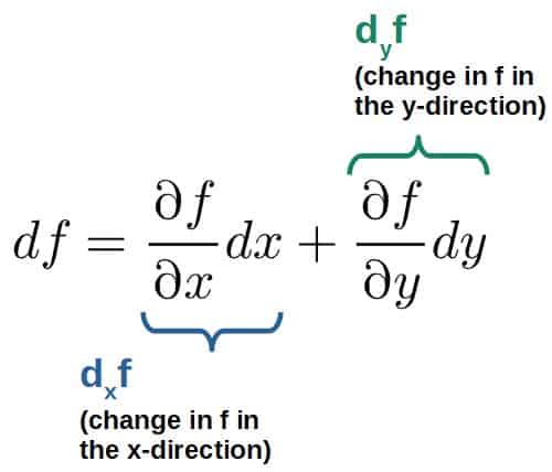
Now, let’s remind ourselves how to calculate the total differential (i.e. change) of a function f(x,y):

Based on this, the changes in r in both the u- and v-directions, d_ur and d_vr, are:

d_uvec{r}=frac{partial vec r}{partial u}du

d_vvec{r}=frac{partialvec{r}}{partial v}dv

Using these, the cross product vector becomes:

dvec{n}=d_uvec{r}times d_vvec{r}=frac{partialvec{r}}{partial u}dutimesfrac{partialvec{r}}{partial v}dv

We can write this expression in the following form:

dvec{n}=frac{partialvec{r}}{partial u}dutimesfrac{partialvec{r}}{partial v}dv=left(frac{partialvec{r}}{partial u}timesfrac{partialvec{r}}{partial v}right)dudv=vec ndudv — Here, I’ve simply used the definition of the normal vector, which is the thing inside of these parentheses.

Now, here comes the key part; the magnitude of a cross product always gives you the area of the parallelogram formed by the vectors you’re taking the cross product of.

So, in this case, if we take the magnitude of this dn-vector, we’ll get the little tiny (infinitesimally tiny, in fact) area spanned by the vectors d_ur and d_vr:

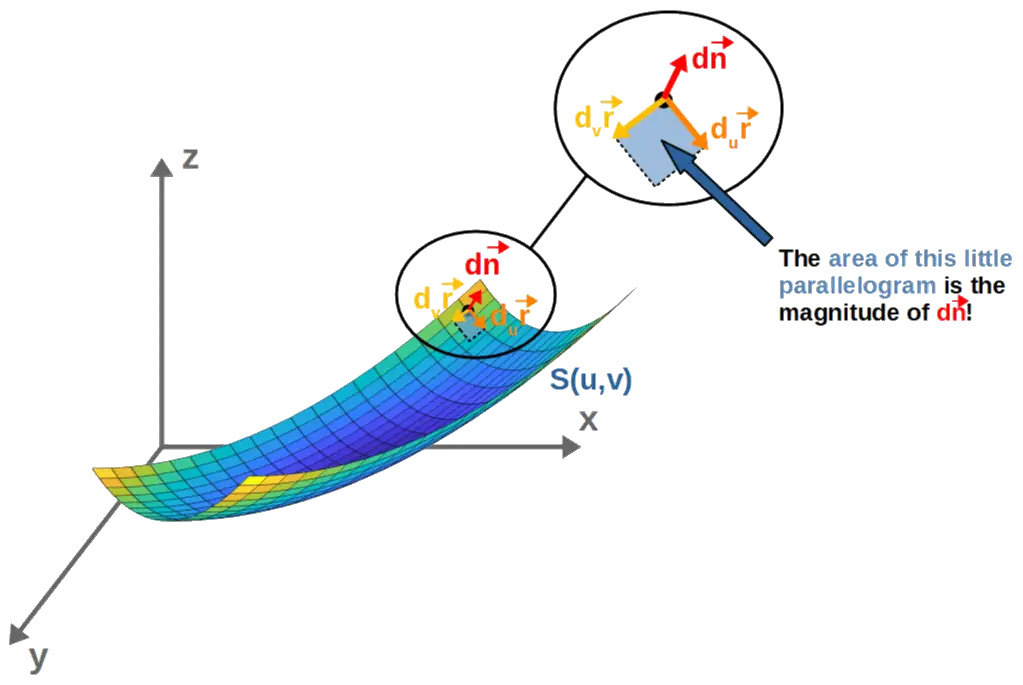
So, the magnitude of the vector dn gives us the area of the parallelogram, which we’ll call dA (since it’s a very very tiny piece of area):

dA=left|dvec{n}right|=left|vec{n}right|dudv

Then, the surface area of this full surface is found simply by adding up all of these little dA’s at each point on the surface!

More mathematically speaking, the surface area of the full surface is obtained by integrating this dA over the surface S (whatever the surface S happens to be):

A=int_{ }^{ }int_S^{ }dA=int_{ }^{ }int_S^{ }left|vec{n}right|dudv — Note that this becomes a double integral, since we’re integrating over both u and v.

So, to put it simply, the steps to to calculate the surface area of a surface are:

Find a suitable u,v-parameterization of the surface. In other words, write your coordinates x, y and z a functions of u and v and form the position vector using these.
Calculate the normal vector to the surface. This is done by differentiating the position vector with respect to both u and v and then taking the cross product of these.
Integrate the magnitude of the normal vector over the surface defined by the parameters u and v.

Example: Surface Area of a Cone

In the last example, we found the normal vector to a cone to be:

To get the surface area of the cone, we first take the magnitude of this:

left|vec{n}right|=sqrt{frac{h^2}{R^2}u^2cos^2v+frac{h^2}{R^2}u^2sin^2v+u^2}

Before integrating, let’s simplify this:

left|vec{n}right|=sqrt{frac{h^2}{R^2}u^2left(cos^2v+sin^2vright)+u^2}=sqrt{frac{h^2}{R^2}u^2+u^2}=sqrt{left(h^2+R^2right)frac{u^2}{R^2}}=sqrt{h^2+R^2}frac{u}{R}

Now, the surface area will be (by integrating this):

A=int_{ }^{ }int_S^{ }left|vec{n}right|dudv=int_{ }^{ }int_S^{ }sqrt{h^2+R^2}frac{u}{R}dudv=frac{1}{R}sqrt{h^2+R^2}int_{ }^{ }int_S^{ }ududv — Here, I’ve pulled out all the constants outside the integral.

Now, this step may be the trickiest as it highly depends on the specific problem we’re trying to solve; we have to define what our surface S actually is.

Luckily for us, this is going to be fairly simple; since u represents the “radius of the bottom circle” of the cone, it’s going to go from 0 to R (the “full radius” of the cone).

On the other hand, v represents the angle around the “bottom circle”, so it will run from 0 to 2π (one full revolution).

Therefore, our surface S is defined by the limits:

The surface integral over S is then:

A=frac{1}{R}sqrt{h^2+R^2}int_{ }^{ }int_S^{ }ududv=frac{1}{R}sqrt{h^2+R^2}int_0^{2pi}int_0^Rududv

This is quite a simple double integral to do. First, let’s integrate with respect to u:

A=frac{1}{R}sqrt{h^2+R^2}int_0^{2pi}int_0^Rududv=frac{1}{R}sqrt{h^2+R^2}int_0^{2pi}frac{u^2}{2}bigg/_{!!!!!0}^Rdv=frac{1}{R}sqrt{h^2+R^2}int_0^{2pi}frac{R^2}{2}dv

Then, pulling out this R²/2, cancelling out one of the R’s and integrating over v, we get:

A=frac{1}{R}sqrt{h^2+R^2}int_0^{2pi}frac{R^2}{2}dv=frac{R}{2}sqrt{h^2+R^2}int_0^{2pi}dv=frac{R}{2}sqrt{h^2+R^2}vbigg/_{!!!!!0}^{2pi}=frac{R}{2}sqrt{h^2+R^2}cdot2pi

So, the full surface area of the cone is:

Note that sometimes you’ll see the surface area of a cone written as:

The difference here is that our formula doesn’t account for the area of the “bottom circle”, πR². If you want the total area of the full cone, you have to add to our formula this factor of πR²:

A_{total}=pi R^2+pi Rsqrt{h^2+R^2}=pi Rleft(R+sqrt{h^2+R^2}right)

Closed Curves & Closed Surfaces

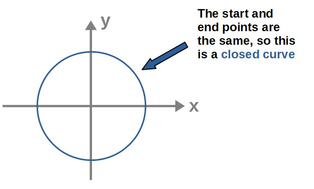
Some particularly important special cases of curves are closed curves. Simply put, these are curves where the start and end points of the curve can be identified as the same point (this then generally makes some sort of closed curve).

Earlier, we used the spiral-like curve as an example; this is an “open” curve, but a circle would be an example of a closed curve:

Now, the important thing about closed curves is that a closed curve always encloses some sort of area or a surface with the boundary of that surface being the curve itself.

This is particularly important for Stokes’ theorem later on, since it relates an integral over a surface to an integral over the boundary of that surface, which of course, has to be a closed curve.

Similarly, we can think of a closed surface as being a surface that encloses some kind of volume. An example of this would be a sphere. In fact, also the cone we looked at earlier is a closed surface if the bottom circle is also taken into account.

We can also think of a closed surface as the boundary to the volume that it is enclosing. This is important when we get to the divergence theorem.

Now, here’s some notation I will be using in the later lessons (though we will come back to these in bit more detail later on):

Surfaces will be denoted by S and their boundaries (the closed curve enclosing that surface) by ∂S. This is a standard piece of notation used in many textbooks.
Volumes will be denoted by V and their boundaries (the closed surface enclosing that volume) by ∂V.
Integrals over closed curves and surfaces will be denoted by an integral symbol with a circle. So, the integral over some closed curve would be denoted by ∮ (instead of the usual ∫-symbol) and the integral over a closed surface would be ∯ (instead of ∬).

Lesson Summary

Here are the key points you should take away from this lesson:

A curve in 3D space can be described parametrically by a single curve parameter (usually denoted t).
Similarly, a surface in 3D space can be described parametrically by two surface parameters (usually denoted u and v).
For a parametric curve, we can calculate its tangent vector at each point along the curve as well as the arc length of the curve from the magnitude of this tangent vector.
For a parametric surface, we can calculate its normal vector at each point on the surface as well as the surface area from the magnitude of this normal vector.
Parametric curves and surfaces can be both open and closed. A closed curve is the boundary of some surface it encloses, while a closed surface is the boundary of some volume it encloses.

Vector Calculus For Physics: A Complete Self-Study Course

Curriculum