Stokes’ Theorem & The Divergence Theorem

The goal of this lesson is to help you understand two of perhaps the most fundamental theorems in vector calculus, Stokes’ theorem and the divergence theorem, as well as what these theorems can be used for.

In the next lesson, we’ll also talk about a third very fundamental theorem to vector calculus known as the Helmholtz decomposition theorem.

Now, to give you some base knowledge, the divergence and Stokes’ theorems have to do with integrating differential operators that act on vector fields (mainly curl and divergence).

We will discover that, in a sense, these theorems are generalizations of the fundamental theorem of calculus that has to do with integrating derivatives.

Lesson Contents

Stokes’ Theorem

In an intuitive sense, Stokes’ theorem relates the properties of a vector field around a closed curve to properties of the vector field inside the closed curve.

So, Stokes’ theorem essentially relates properties of a vector field in some region to properties of the field at the boundary of that region (this is actually what the divergence theorem does as well).

More specifically, Stokes’ theorem states that the total circulation of a vector field around a closed curve can be expressed by adding up the total “circulation” of the vector field inside of the curve.

As a reminder, the circulation of a vector field was defined as the line integral over a closed curve:

Now, by total “circulation” inside of the curve, I’m essentially talking about adding up each of the “local circulation densities” in this region bounded by the closed curve (the “local circulation densities” meaning the curl of the vector field at each point, like we talked about in the lesson on the curl operator).

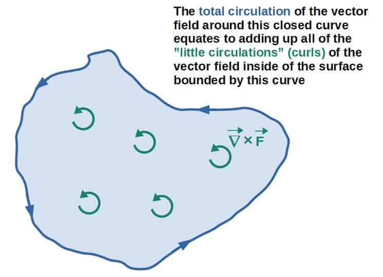
This is drawn in 2D for simplicity. Note, however, that the curve, in general, is going to be in 3D so the surface will also.

Mathematically, this can be expressed as the circulation around a closed curve being equal to the surface integral of the curl inside of the curve:

oint_gammavec{F}cdot dvec{r}=iint_S(vec{nabla}timesvec{F})cdot vec ndS

This right here is exactly Stokes’ theorem. It is this equation which relates a circulation integral to a flux integral.

Now, one nice thing about Stokes’ theorem is that it’s very general. In fact, Stokes’ theorem can easily be generalized to “higher-dimensional” surfaces called manifolds, which are actually used to model spacetime in Einstein’s theory of general relativity.

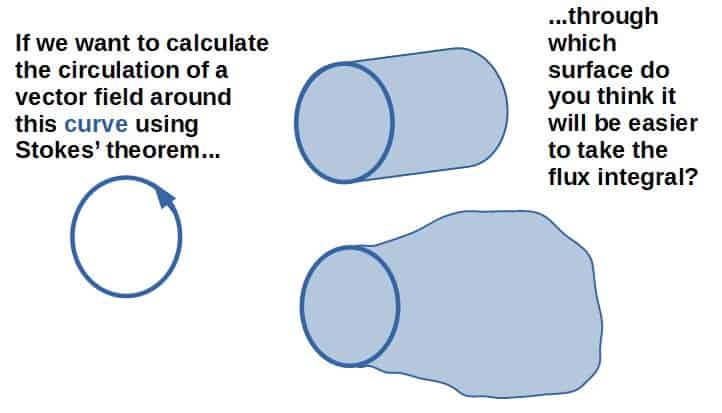
Another useful thing about Stokes’ theorem is that it allows us to calculate the line integral of a vector field around a closed loop simply by 1) taking the curl of a vector field and 2) calculating the flux integral of this curl vector through a surface.

However, what makes this incredibly powerful is that the surface you define for the flux integral can be any surface, as long as it has the specific curve as a boundary.

We can therefore greatly simplify many calculations just by choosing the right surface to take the flux integral through. This is illustrated in the picture below.

Example of Using Stokes' Theorem

The goal of this example will be to illustrate how Stokes’ theorem can be used to mathematically simplify certain problems.

Now, let’s say we have the following vector field:

vec{F}left(x{,}y{,}zright)=frac{1}{2}y^2xhat{x}+frac{xz}{1+cos^2y}hat{y}+e^{x^2z}hat{z}

We now want to calculate the circulation of this vector field around the parallelogram in the xy-plane with vertices (0,0), (a,b), (c,b) and (d,0):

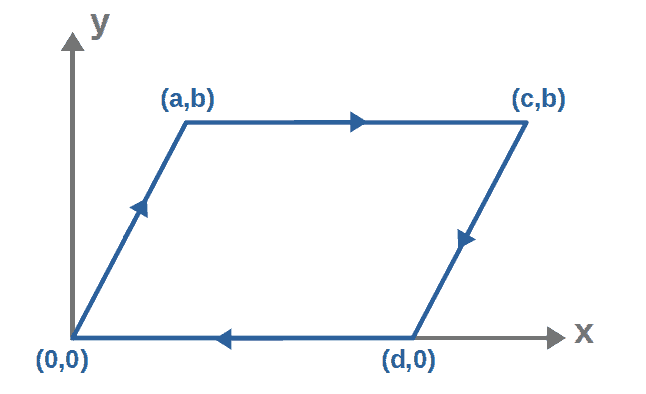
The circulation would be calculated by the following closed line integral:

oint_{gamma}^{ }vec{F}cdot dvec{r}=oint_{gamma}^{ }vec{F}cdotfrac{dvec{r}}{dt}dt

In general, to do this closed line integral, we’d have to divide the line integral into four curves (one along each side), parameterize each curve and then calculate four different integrals, which can be a little tedious.

Instead, since we have a circulation integral, we can simply apply Stokes’ theorem, which states that calculating the circulation is equivalent to calculating the following surface integral:

oint_{gamma}^{ }vec{F}cdot dvec{r}=iint_S^{ }left(vec{∇}timesvec{F}right)cdotvec{n}dS

We’ll see that calculating this surface integral is actually quite easy. The first thing we have to do is actually choose the surface, which has to have to sides of the parallelogram as its boundary. Well, we can simply just choose the surface of the parallelogram as our surface to integrate along:

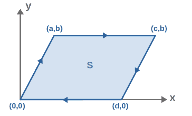
To calculate the surface integral, we first have to parameterize our surface S as S(u,v). One way to do this is by choosing two surface parameters, u and v, such that they both run from 0 to 1. Doing this, we can express any point on this surface according to the picture below:

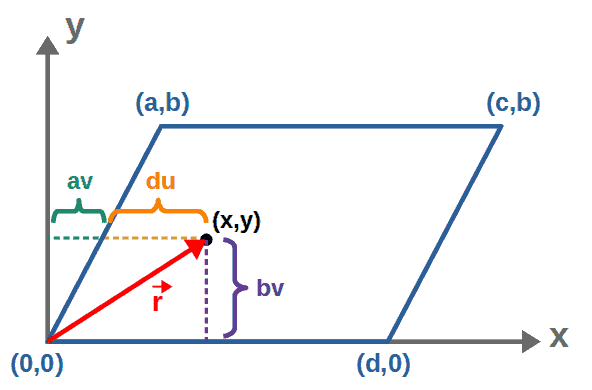
These u and v parameters can, in a sense, be thought of as “percentages” since they both run from 0 to 1, meaning that for example, v=1, u=0 would correspond to the point (a,b) since this point could be expressed “0% in terms of the parameter u and 100% in terms of the parameter v”.

So, the coordinates x and y of any point on the surface can be expressed in terms of these parameters as:

The position vector of this point is then:

vec{r}left(u{,}vright)=left(av+duright)hat{x}+bvhat{y}

Taking the partial derivatives of this, we have:

frac{partialvec{r}}{partial u}=dhat{x}+0hat{y}

frac{partialvec{r}}{partial v}=ahat{x}+bhat{y}

The normal vector to this surface is then:

vec{n}=frac{partialvec{r}}{partial u}timesfrac{partialvec{r}}{partial v}=0hat{x}+0hat{y}+left(bcdot d-0cdot aright)hat{z}=bdhat{z} — Technically, the cross product is only defined in 3D, but we can just imagine that the position vector is a 3D vector with its z-component begin zero.

We also need the curl of our vector field. Now, because the normal vector only has a z-component and the surface integral consists of a dot product, only the z-component of the curl will play a role (since the other terms in the dot product will be zero).

The z-component of our curl is:

left(vec{∇}timesvec{F}right)_z=frac{partial F_y}{partial x}-frac{partial F_x}{partial y}=frac{z}{1+cos^2y}-yx

Now, before doing the surface integral, we need to express this in terms of our parameterization:

Inserting these, the z-component of the curl becomes:

left(vec{∇}timesvec{F}right)_z=0-bvleft(av+duright)=-abv^2-bduv

So, using everything we have so far, our surface integral becomes:

iint_S^{ }left(vec{∇}timesvec{F}right)cdotvec{n}dS=int_0^1int_0^1left(-abv^2-bduvright)bddudv=-int_0^1int_0^1left(ab^2dv^2+b^2d^2uvright)dudv — As a reminder, earlier we took the parameters u and v to go from 0 to 1, which is where these limits of integration come from.

Doing the integral over u first, we get:

-int_0^1int_0^1left(ab^2dv^2+b^2d^2uvright)dudv=-int_0^1bigg/_{!!!!!0}^1left(ab^2dv^2u+b^2d^2frac{u^2}{2}vright)dv=-int_0^1left(ab^2dv^2+frac{1}{2}b^2d^2vright)dv

Then, from the v-integral, we have:

-int_0^1left(ab^2dv^2+frac{1}{2}b^2d^2vright)dv=-bigg/_{!!!!!0}^1left(ab^2dfrac{v^3}{3}+frac{1}{2}b^2d^2frac{v^2}{2}right)=-left(frac{1}{3}ab^2d+frac{1}{4}b^2d^2right)

All in all, we then have that the surface integral is:

iint_S^{ }left(vec{∇}timesvec{F}right)cdotvec{n}dS=-frac{b^2}{12}left(4ad+3d^2right)

Now, the whole purpose of this was to calculate the circulation, after all. By Stokes’ theorem, the circulation integral is the same as this surface integral we just calculated. So, the answer to our problem is then:

oint_{gamma}^{ }vec{F}cdot dvec{r}=-frac{b^2}{12}left(4ad+3d^2right)

This may have seemed like a much more complicated way to calculate the circulation integral, but actually, this was probably a much simpler and faster calculation than it would have been to calculate the actual line integral around the parallelogram.

Sidenote; in vector calculus, you'll often come across something called Green's theorem. The reason we're not discussing Green's theorem explicitly is because it is just a special case of Stokes' theorem, namely Stokes' theorem in 2D (on the xy-plane).

Applications of Stokes’ Theorem In Physics

Some of the more interesting applications of Stokes’ theorem actually come from physics and I think it’s relevant to discuss these here.

One example in physics comes from the notion of a conservative force, in particular, the way a conservative force can be defined in terms of a potential.

A conservative force can be modeled by a path independent vector field. In vector calculus language, this means that for a path independent vector field, the circulation around any closed curve is always zero:

If we apply Stokes’ theorem here, we get a condition for such a vector field:

oint_{gamma}vec{F}cdot dvec{r}=iint_S(vec{∇}timesvec{F})cdot vec ndS=0 Rightarrow vec{∇}timesvec{F}=0

In other words, a conservative force field in physics is a vector field with zero curl.

Now, it is also a well-known result that the curl of the gradient of any scalar field is zero. Therefore, we can write a conservative force as the gradient of a scalar field and it will satisfy this condition of path independence:

vec{∇}timesvec{F}=0 Leftrightarrow vec{F}=-vec{∇}U — It is conventional to put a minus sign here. This is most commonly seen in physics.

This scalar field U here is the potential energy. Notice that this relationship between a conservative force and potential energy is simply a result of Stokes’ theorem.

The same is NOT true for a non-conservative force since they are generally not path independent. If you’re interested in more about this topic, I have a full article on this on my website.

Another useful application of Stokes’ theorem in physics is for converting between differential and integral forms of certain equations.

The most famous example of this is with Maxwell’s equations of electromagnetism. The four Maxwell equations can essentially be expressed in both integral and differential forms. You can see these from the table below.

∯_Svec{E}cdotvec{n}dS=frac{Q_{tot}}{varepsilon_0}

vecnablacdot vec E=frac{rho}{varepsilon_0}

Maxwell Equation	Integral Form	Differential Form
Gauss’s law (for the electric field)	$∯_Svec{E}cdotvec{n}dS=frac{Q_{tot}}{varepsilon_0}$	$vecnablacdot vec E=frac{rho}{varepsilon_0}$
Gauss’s law (for the magnetic field)	$∯_Svec{B}cdotvec{n}dS=0$	$vec{∇}cdot vec B=0$
Faraday’s law	$oint_{gamma}^{ }vec{E}cdot dvec{r}=-frac{d}{dt}iint_S^{ }vec{B}cdotvec{n}dS$	$vec{∇}timesvec{E}=-frac{partial vec B}{partial t}$
Ampere’s law	$oint_{gamma}^{ }vec{B}cdot dvec{r}=mu_0iint_S^{ }vec{J}cdotvec{n}dS+mu_0varepsilon_0frac{d}{dt}iint_S^{ }vec{E}cdotvec{n}dS$	$vec{∇}timesvec{B}=mu_0vec{J}+mu_0varepsilon_0frac{partialvec{E}}{partial t}$

The main use of this “convertion” between the integral and differential forms is that the integral forms can be applied easily in highly symmetric situations and they tell us about the behaviour of the electric and magnetic fields in an intuitive sense.

On the other hand, the differential forms of the Maxwell equations give us differential equations that we may want to solve for the components of the E- and B -fields. This can be used in any situation, not just in highly symmetric cases.

The way to actually convert between the integral and differential forms is by applying Stokes’ theorem and also the divergence theorem (which we’ll talk about soon). You’ll find examples of how to actually do this down below.

Faraday's Law and Ampere's Law Using Stokes' Theorem

From the four Maxwell equations, Faraday’s law and Ampere’s law can be converted from the integral to the differential form (or vice versa) using Stokes’ theorem. The two Gauss’s laws are converted using the divergence theorem, which we’ll see later.

Let’s begin by looking at Faraday’s law from the integral form:

oint_{gamma}^{ }vec{E}cdot dvec{r}=-frac{d}{dt}iint_S^{ }vec{B}cdotvec{n}dS

On the left-hand side, we have a circulation integral, so we can apply Stokes’ theorem here. Faraday’s law then becomes:

oint_{gamma}^{ }vec{E}cdot dvec{r}=iint_S^{ }left(vec{∇}timesvec{E}right)cdotvec{n}dS Rightarrow iint_S^{ }left(vec{∇}timesvec{E}right)cdotvec{n}dS=-frac{d}{dt}iint_S^{ }vec{B}cdotvec{n}dS

By assumption, we’ll take Faraday’s law to apply to surfaces that themselves don’t change with time (i.e. the integration limits on the right-hand side are time independent). We can therefore move the d/dt inside the integral sign to act on the B-field provided that it becomes a partial derivative:

iint_S^{ }left(vec{∇}timesvec{E}right)cdotvec{n}dS=-iint_S^{ }frac{partialvec{B}}{partial t}cdotvec{n}dS

Since these are both flux integrals (through the same surface S), we can conclude that for this equality to hold generally, the integrands have to be equal. We then get Faraday’s law in differential form:

vec{∇}timesvec{E}=-frac{partialvec{B}}{partial t}

Similarly, we can also do the same for Ampere’s integral law:

oint_{gamma}^{ }vec{B}cdot dvec{r}=mu_0iint_S^{ }vec{J}cdotvec{n}dS+mu_0varepsilon_0frac{d}{dt}iint_S^{ }vec{E}cdotvec{n}dS

Let’s begin by applying Stokes’ theorem on the left-hand side, which will give us:

iint_S^{ }(vec{∇}timesvec{B})cdotvec{n}dS=mu_0iint_S^{ }vec{J}cdotvec{n}dS+mu_0varepsilon_0frac{d}{dt}iint_S^{ }vec{E}cdotvec{n}dS

By the same logic as earlier, we can move the d/dt inside the integral sign provided that it becomes a partial derivative acting on E. We then get:

iint_S^{ }(vec{∇}timesvec{B})cdotvec{n}dS=mu_0iint_S^{ }vec{J}cdotvec{n}dS+mu_0varepsilon_0iint_S^{ }frac{partial vec{E}}{partial t}cdotvec{n}dS

Again, for this to generally hold, we have to have all of the integrands equal to each other, so we get Ampere’s law in differential form:

vec{∇}timesvec{B}=mu_0vec{J}+mu_0varepsilon_0frac{partialvec{E}}{partial t}

The Divergence Theorem

Similarly to Stokes’ theorem, the divergence theorem also relates properties of a vector field inside “something” to the properties of a vector field at the boundary of that “something”.

Now, Stokes’ theorem was used to relate a closed line integral (circulation) to a surface integral. In contrast, the divergence theorem is used to relate a closed surface integral (flux) to a volume integral.

More specifically, the divergence theorem states that the total flux of a vector field through a closed surface can be calculated by adding up all of the little “sources” (the divergence at each point) inside of the closed surface.

To avoid clutter and give you an intuitive picture, I’ve drawn this in 2D. However, what you should really picture in your head is this V being a volume in 3D with this S being its surface boundary.

Mathematically, the way to state this would be that the flux integral of a vector field is equal to the volume integral of the divergence of that vector field (i.e. we’re “adding up” the divergence at each point over the whole volume):

∯_Svec{F}cdotvec{n}dS=iiint_V^{ }left(vec{∇}cdotvec{F}right)dV

As we saw with Stokes’ theorem, the divergence theorem can also be used to simplify calculations.

Also, the nice thing about the divergence theorem is that it allows us to avoid the whole process of parameterizing a surface when calculating the flux of a vector field.

Instead, we can simply take the divergence of the vector field and then calculate an ordinary triple integral. In a lot of cases, this will be much faster than parameterizing a surface, finding its normal vector and so on.

Now, the only restriction for this is that the divergence theorem only applies to closed surfaces that enclose some volume.

Example of Using The Divergence Theorem

One of the more common examples of applying the divergence theorem is for the case when we have a geometry (such as a cube) that is composed of multiple sides.

For our example, we’ll take a cube of side length a (with one of its corners being in the origin):

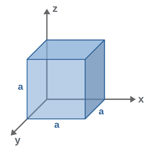
We then want to calculate the total flux through the surface of the cube of the following vector field:

vec{F}left(x{,}y{,}zright)=left(1+zcos yright)e^yhat{x}+frac{1}{2}x^2y^2hat{y}+sqrt{1+z^2}hat{z}

In this case, calculating the total flux through the surface would require calculating the flux through each side individually as each of the sides would have a different parameterization. This can be somewhat tedious at it requires doing six different integrals and finding six different parameterizations.

Luckily, we have the divergence theorem at hand, which states that the total flux of the vector field through the cube’s surface is the same as the volume integral of the divergence of this vector field:

A volume integral over a cube is generally going to be quite easy to calculate.

The nice thing about this is that we do not even need to parameterize anything, unlike if we were to actually calculate the flux integral itself.

All we really need is the divergence of our vector field, which will be:

vec{∇}cdotvec{F}=frac{partial F_x}{partial x}+frac{partial F_y}{partial y}+frac{partial F_z}{partial z}=0+x^2y+frac{z}{sqrt{1+z^2}}

So, the right-hand side of the divergence theorem is then:

iiint_V^{ }left(vec{∇}cdotvec{F}right)dV=int_0^aint_0^aint_0^aleft(x^2y+frac{z}{sqrt{1+z^2}}right)dxdydz — These integration limits come from the fact that each side of the cube runs from 0 to a.

Let’s do the x-integral first:

int_0^aint_0^aint_0^aleft(x^2y+frac{z}{sqrt{1+z^2}}right)dxdydz=int_0^aint_0^abigg/_{!!!!!0}^aleft(frac{x^3}{3}y+frac{xz}{sqrt{1+z^2}}right)dydz=int_0^aint_0^aleft(frac{a^3}{3}y+frac{az}{sqrt{1+z^2}}right)dydz

Then the y-integral:

int_0^aint_0^aleft(frac{a^3}{3}y+frac{az}{sqrt{1+z^2}}right)dydz=int_0^abigg/_{!!!!!0}^aleft(frac{a^3}{3}frac{y^2}{2}+frac{azy}{sqrt{1+z^2}}right)dz=int_0^aleft(frac{a^5}{6}+frac{a^2z}{sqrt{1+z^2}}right)dz

Let’s split this integral into two parts:

int_0^aleft(frac{a^5}{6}+frac{a^2z}{sqrt{1+z^2}}right)dz=bigg/_{!!!!!0}^afrac{a^5}{6}z+a^2int_0^afrac{z}{sqrt{1+z^2}}dz=frac{a^6}{6}+a^2int_0^afrac{z}{sqrt{1+z^2}}dz

Let’s now focus specifically on the last integral here:

We can do a simple u-substitution and calculate dz from it:

Let’s look at how the integration limits change. When we have z=0, the corresponding u-limit will be:

For the limit z=a, we have:

Using all of these, the integral now becomes:

int_0^afrac{z}{sqrt{1+z^2}}dz Rightarrow int_1^{1+a^2}frac{z}{sqrt{u}}cdotfrac{1}{2z}du=frac{1}{2}int_1^{1+a^2}frac{1}{sqrt{u}}du

This integral gives us simply (by using 1/√u=u^-1/2):

frac{1}{2}int_1^{1+a^2}frac{1}{sqrt{u}}du=frac{1}{2}bigg/_{!!!!!1}^{1+a^2}2sqrt{u}=sqrt{1+a^2}-1

Substituting this result back into our original expression, we then have:

frac{a^6}{6}+a^2int_0^afrac{z}{sqrt{1+z^2}}dz=frac{a^6}{6}+a^2left(sqrt{1+a^2}-1right)

Now, this is the volume integral of the divergence. So, by the divergence theorem this is also the total flux of the vector field through the surfaces of the cube and we have our answer:

∯_Svec{F}cdotvec{n}dS=frac{a^6}{6}+a^2left(sqrt{1+a^2}-1right)

As you can see, this was a fairly simple calculation. We just had to 1) take the divergence of our vector field and 2) calculate a fairly easy triple integral.

In contrast, we could have calculated the actual flux integral by 1) parameterizing all six sides of the cube, 2) calculating the normal vector to each side and 3) calculating six different flux integrals. Which do you think was the easier method?

Applications of The Divergence Theorem In Physics

The divergence theorem also has plenty of applications in physics. The most well-known application is probably for converting Maxwell’s equations from integral to differential form, similarly to how Stokes’ theorem was used.

Specifically, the divergence theorem can be used to convert the two Gauss’s laws (both for the electric and magnetic fields). You’ll see how this is done below.

The divergence theorem can also be used to convert between the integral and differential forms of the continuity equation, which basically describes the conservation of electric charge in classical electrodynamics. This is done in one of the practice problems in your problem set.

Gauss's Law For The Electric and Magnetic Fields Using The Divergence Theorem

For this example, we want to convert Gauss’s laws for both the electric and the magnetic field from the integral form to the differential form (since in most textbooks, these laws are first introduced in their integral forms).

Let’s begin with Gauss’s law for the magnetic field, which is the simpler case:

Now, you may want to ask whether we could just conclude right away from this that B=0?

We can’t, since this is a dot product and moreover, an integral over a closed surface (which means that this only describes the total flux over the whole surface). Due to this, we cannot necessarily conclude much about the integrand itself.

So, we therefore need to convert this into a “non-closed integral”, which can be done using the divergence theorem. Applying that, we can turn this closed surface integral into a volume integral of the form (the right-hand side still being zero, of course):

∯_Svec{B}cdotvec{n}dS=iiint_V^{ }left(vec ∇cdot vec Bright)dV=0

Since this is an integral over an “open domain” and it is equal to zero, it must follow that the integrand has to be zero:

iiint_V^{ }left(vec{∇}cdotvec{B}right)dV=0 Rightarrow vec{∇}cdotvec{B}=0

This is, of course, Gauss’s law in its differential form.

We can repeat the same process for the electric field, only now the right-hand side in Gauss’s integral law is not zero but rather has the total charge (inside of the closed surface S):

Now, this total charge inside of the closed surface is simply the “charge density times the volume enclosed by the surface”. In integral language, this would be the volume integral of the charge density (as this density may be a function of position, generally speaking):

Gauss’s law can then be expressed as:

∯_Svec{E}cdotvec{n}dS=iiint_V^{ }frac{rho}{varepsilon_0}dV

We can now apply the divergence theorem to the left-hand side. The surface integral on the left-hand side will then turn into the volume integral over the volume enclosed by this closed surface, which is the same volume V as we have on the right-hand side as well:

∯_Svec{E}cdotvec{n}dS=iiint_V^{ }frac{rho}{varepsilon_0}dV Rightarrow iiint_V^{ }left(vec{∇}cdotvec{E}right)dV=iiint_V^{ }frac{rho}{varepsilon_0}dV

Since these are now expressed as integrals over the same domain (the volume V here), it follows that the integrands have to be equal:

iiint_V^{ }left(vec{∇}cdotvec{E}right)dV=iiint_V^{ }frac{rho}{varepsilon_0}dV Rightarrow vec{∇}cdotvec{E}=frac{rho}{varepsilon_0}

And that’s just Gauss’s law in differential form! Hopefully this demonstrates the application of the divergence theorem to physics and why it’s so useful.

There are also plenty more examples similar to this where the divergence theorem is used to essentially “convert” certain equations and physical laws into different forms.

Another notable application of the divergence theorem comes from the notion of an incompressible vector field. To put it simply, an incompressible vector field is a vector field that has zero net flux through any closed surface:

The intuition for this comes from the fact that if the net flux through a closed surface is zero, there is always “as much” of the vector field flowing into the surface as there is flowing out of the surface. Thus, the vector field is said to be “incompressible”.

Now, the divergence theorem allows us to deduce an equivalent condition for an incompressible vector field. If we apply the divergence theorem to the closed surface integral given above, we get the following condition:

∯_Svec{F}cdotvec{n}dS=iiint_V^{ }left(vec{∇}cdotvec{F}right)dV=0 Rightarrow vec{∇}cdotvec{F}=0

Therefore, an incompressible vector field always has zero divergence.

Now, remember that any curl-free vector field could be written as the gradient of a scalar potential. Similarly, any divergence-free vector field can be written as the curl of a vector potential:

This follows directly from the fact that generally, the divergence of the curl of any vector field is always zero.

In terms of how this applies to physics, one example comes from electrodynamics. Essentially, Gauss’s law for a magnetic field states that the divergence of a magnetic field is always zero:

In other words, all magnetic fields are incompressible vector fields. Therefore, any magnetic field can also be written in terms of a magnetic vector potential as:

Another example comes from the notion of incompressible fluid flow. In general, incompressible fluid flow is defined by the flow velocity of the fluid being divergence-free:

This can also be written as the curl of a vector potential, which is often called a stream function. Now, a stream function is usually only defined for 2D fluid flow (since it’s not a particularly useful concept in 3D), in which case the stream function would be:

vec psi=psileft(x{,}yright)hat{z} — In other words, this stream function is a vector field with its x and y components being zero and the z-component being ψ(x,y).

Then, the velocity field for incompressible flow can be written in terms of this stream function as:

vec{u}=vec{∇}timesvec{psi}=frac{partialpsi}{partial y}hat{x}-frac{partialpsi}{partial x}hat{y}

The divergence theorem also has applications in differential geometry. In fact, the divergence theorem for a vector field can be generalized to curved spaces, in which case it wold have the following form:

∯_SF^in_isqrt{left|gammaright|}dS=iiint_V^{ }partial_ileft(sqrt{left|gright|}V^iright)dV — Note; this ‘index notation’ is explained in detail in one of the later lessons in this course.

Now, this may look complicated but the content is really the same; on the left, we have an integral over a 2D surface and on the right, a 3D volume integral of the divergence.

Without getting into the details, in a curved space, we also have to throw in these factors of metric determinants (g) and an induced metric determinant (γ). Moreover, this thing on the right is essentially the “covariant divergence”, a more general form of the divergence.

This can actually be used in general relativity to define conservation laws in some cases. In special cases of certain “spacetime symmetries”, it is possible to define conserved quantities (such as energy or angular momentum).

If this is the case, it’s possible to essentially write an integral form of a conservation law for these quantities using the divergence theorem in curved spacetime:

oint_{partial V}T^{munu}xi_{nu}n_{mu}sqrt{left|gammaright|}d^3x=int_V^{ }partial_{mu}left(sqrt{left|gright|}T^{munu}xi_{nu}right)d^4x — This T^µν here is the energy-momentum tensor, which represents sources of gravity in general relativity. This ξ_ν is something called a Killing vector, which is essentially used to represent conserved quantities in spacetime.

While this may look confusing, we essentially have a 4D (spacetime) volume integral over a divergence on the right and a closed surface integral on the left (the closed surface being a 3D volume, which encloses the 4D volume).

Now, these are just examples of some higher-level applications of the divergence theorem to whet your appetite for learning this stuff, since you may encounter these once you get further in your physics and math learning journey.

What Is The Big Picture With These Theorems?

We’ve now covered Stokes’ theorem and the divergence theorem, two theorems that many would call the cornerstones of vector calculus (there is actually one more fundamental theorem in vector calculus that we’ll talk about in the next lesson).

Now, both of these theorems are useful in their own sense and have many applications, but I’d like to encourage you to think bigger here. Namely, about the big picture with these theorems.

Sure, these are just two theorems, but actually, under these theorems there is an extremely elegant and deep geometric idea that goes far beyond just vector calculus.

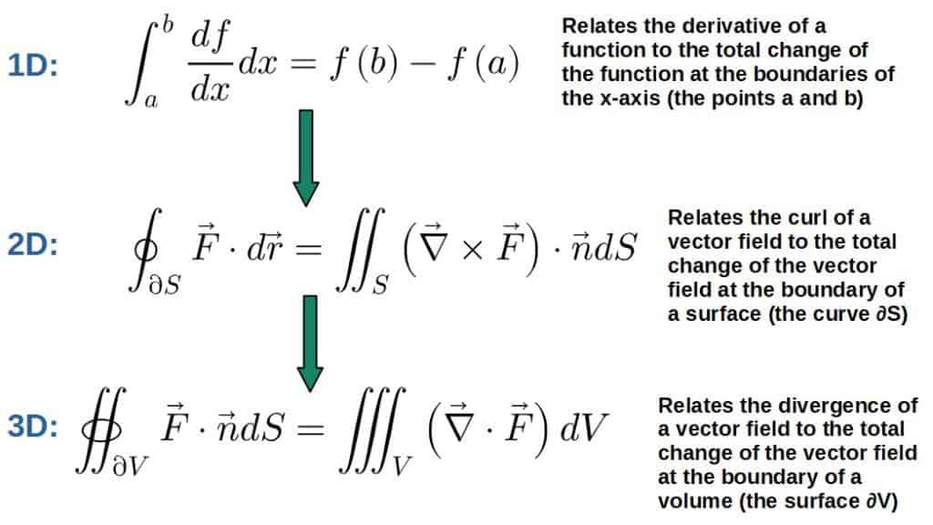
To understand this, we need to go way back to the fundamental theorem of calculus:

int_a^bfrac{df}{dx}dx=fleft(bright)-fleft(aright)

The usual way of interpreting this is that integrating a derivative of a function gives you back the function itself or in other words, that integrals and derivatives are “opposite” operations of one another.

However, this is actually not a very good way of thinking about the fundamental theorem of calculus.

How you would really want to think about it is as follows; adding up all of the little changes of a function gives you the total change in the function at the boundaries.

Put more mathematically, integrating a differential of something gives you the total change in that something at the boundaries.

Well, this is exactly what both Stokes’ theorem and the divergence theorem tells you; Stokes’ theorem gives you the total circulation of a vector field around the boundary of a surface by adding up the curl of the vector field at each point inside the surface.

Moreover, the divergence theorem gives you the total flux of a vector field through the boundary of a volume by adding up the divergence of the vector field at each point inside the volume.

So, in fact, both Stokes’ theorem and the divergence theorem are just higher-dimensional generalizations of the fundamental theorem of calculus, which is best thought of as stating that integrals and derivatives are NOT opposites of each other, but rather relate local changes in something to global changes in that something.

Now, in mathematics at least, it’s common to want to generalize things to even higher dimensions. What would the fundamental theorem of calculus look like in 4D?

This is where the generalized Stokes’ theorem comes in, which is in a sense, one of the most important theorems in all of calculus.

The Generalized Stokes’ Theorem

The generalized Stokes’ theorem, as the name may suggest, generalizes Stokes’ theorem to higher dimensions.

However, the generalized Stokes’ theorem also generalizes the divergence theorem, the fundamental theorem of calculus and pretty much all of the integral theorems of vector calculus into one big equation.

Well, actually the equation describing the generalized Stokes’ theorem is not big at all:

int_M^{ }domega=int_{partial M}^{ }omega

It may be hard to believe, but this single equation actually encompasses the divergence theorem, Stokes’ theorem and all other relevant theorems.

Now, what does this actually mean?

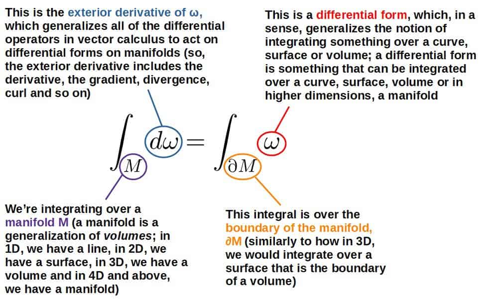
In a nutshell, the generalized Stokes’ theorem says that integrating the exterior derivative (a “local change”) of a differential form over a manifold is equivalent to integrating the differential form itself over the boundary of the manifold (adding up to a “global change” at the boundaries).

Or stated even simpler, adding up small changes inside a manifold equates to the total change at the boundary of the manifold.

This is exactly what all the other integral theorems in vector calculus say, this just generalizes that statement even further!

Indeed, the generalized Stokes’ theorem is one of the most powerful theorems in calculus and that’s because it’s so general; in mathematics, it is not often that such a general and unifying theorem is discovered.

In practice, the general Stokes’ theorem has uses in differential geometry, among other things.

Differential geometry and manifolds, on the other hand, can be applied to general relativity in the form of spacetime (a 4D manifold) and the curvature of spacetime. So, the generalized Stokes’ theorem works even in general relativity when dealing with curved spacetime describing gravity.

Vector Calculus For Physics: A Complete Self-Study Course

Curriculum